Note
Go to the end to download the full example code.
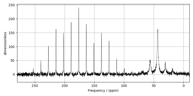
¹³C MAS NMR of Glycine (CSA) [960 Hz]
The following is a sideband least-squares fitting example of a \(^{13}\text{C}\) MAS NMR spectrum of Glycine spinning at 960 Hz. The following experimental dataset is a part of DMFIT [1] examples. We thank Dr. Dominique Massiot for sharing the dataset.
import csdmpy as cp
import numpy as np
import matplotlib.pyplot as plt
from lmfit import Minimizer

from mrsimulator import Simulator, SpinSystem, Site
from mrsimulator.method.lib import BlochDecaySpectrum
from mrsimulator import signal_processor as sp
from mrsimulator.utils import spectral_fitting as sf
from mrsimulator.utils import get_spectral_dimensions
Import the dataset
host = "https://nmr.cemhti.cnrs-orleans.fr/Dmfit/Help/csdm/"
filename = "13C MAS 960Hz - Glycine.csdf"
experiment = cp.load(host + filename)

# For spectral fitting, we only focus on the real part of the complex dataset
experiment = experiment.real

# Convert the coordinates along each dimension from Hz to ppm.
_ = [item.to("ppm", "nmr_frequency_ratio") for item in experiment.dimensions]

# plot of the dataset.
plt.figure(figsize=(8, 4))
ax = plt.subplot(projection="csdm")
ax.plot(experiment, color="black", linewidth=0.5, label="Experiment")
ax.set_xlim(280, -10)
plt.grid()
plt.tight_layout()
plt.show()
Estimate noise statistics from the dataset
coords = experiment.dimensions[0].coordinates
noise_region = np.where(coords < 10e-6)
noise_data = experiment[noise_region]

plt.figure(figsize=(3.75, 2.5))
ax = plt.subplot(projection="csdm")
ax.plot(noise_data, label="noise")
plt.title("Noise section")
plt.axis("off")
plt.tight_layout()
plt.show()

noise_mean, sigma = experiment[noise_region].mean(), experiment[noise_region].std()
noise_mean, sigma
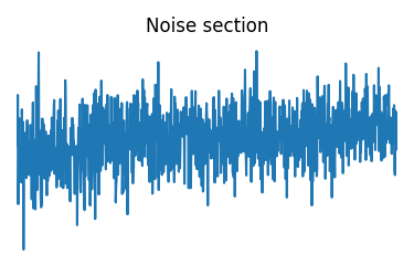
(<Quantity 0.6193483>, <Quantity 3.939941>)
Create a fitting model
Spin System
C1 = Site(
    isotope="13C",
    isotropic_chemical_shift=176.0,  # in ppm
    shielding_symmetric={"zeta": 70, "eta": 0.6},  # zeta in Hz
)
C2 = Site(
    isotope="13C",
    isotropic_chemical_shift=43.0,  # in ppm
    shielding_symmetric={"zeta": 30, "eta": 0.5},  # zeta in Hz
)

spin_systems = [SpinSystem(sites=[C1], name="C1"), SpinSystem(sites=[C2], name="C2")]
Method
# Get the spectral dimension parameters from the experiment.
spectral_dims = get_spectral_dimensions(experiment)

MAS = BlochDecaySpectrum(
    channels=["13C"],
    magnetic_flux_density=7.05,  # in T
    rotor_frequency=960,  # in Hz
    spectral_dimensions=spectral_dims,
    experiment=experiment,  # experimental dataset
)
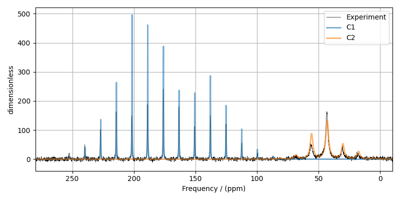
Guess Model Spectrum
# Simulation
# ----------
sim = Simulator(spin_systems=spin_systems, methods=[MAS])
sim.config.decompose_spectrum = "spin_system"
sim.run()

# Post Simulation Processing
# --------------------------
processor = sp.SignalProcessor(
    operations=[
        sp.IFFT(),
        sp.apodization.Exponential(FWHM="20 Hz", dv_index=0),  # spin system 0
        sp.apodization.Exponential(FWHM="200 Hz", dv_index=1),  # spin system 1
        sp.FFT(),
        sp.Scale(factor=1000),
    ]
)
processed_dataset = processor.apply_operations(dataset=sim.methods[0].simulation).real

# Plot of the guess Spectrum
# --------------------------
plt.figure(figsize=(8, 4))
ax = plt.subplot(projection="csdm")
ax.plot(experiment, color="black", linewidth=0.5, label="Experiment")
ax.plot(processed_dataset, linewidth=2, alpha=0.6)
ax.set_xlim(280, -10)
plt.grid()
plt.legend()
plt.tight_layout()
plt.show()
Least-squares minimization with LMFIT
Use the make_LMFIT_params() for a quick
setup of the fitting parameters.
params = sf.make_LMFIT_params(sim, processor, include={"rotor_frequency"})
print(params.pretty_print(columns=["value", "min", "max", "vary", "expr"]))
Name                                      Value      Min      Max     Vary     Expr
SP_0_operation_1_Exponential_FWHM            20     -inf      inf     True     None
SP_0_operation_2_Exponential_FWHM           200     -inf      inf     True     None
SP_0_operation_4_Scale_factor              1000     -inf      inf     True     None
mth_0_rotor_frequency                       960      860     1060     True     None
sys_0_abundance                              50        0      100     True     None
sys_0_site_0_isotropic_chemical_shift       176     -inf      inf     True     None
sys_0_site_0_shielding_symmetric_eta        0.6        0        1     True     None
sys_0_site_0_shielding_symmetric_zeta        70     -inf      inf     True     None
sys_1_abundance                              50        0      100    False 100-sys_0_abundance
sys_1_site_0_isotropic_chemical_shift        43     -inf      inf     True     None
sys_1_site_0_shielding_symmetric_eta        0.5        0        1     True     None
sys_1_site_0_shielding_symmetric_zeta        30     -inf      inf     True     None
None
Solve the minimizer using LMFIT
opt = sim.optimize()
minner = Minimizer(
    sf.LMFIT_min_function,
    params,
    fcn_args=(sim, processor, sigma),
    fcn_kws={"opt": opt},
)
result = minner.minimize()
result
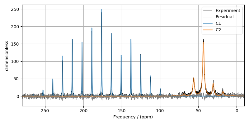
The best fit solution
best_fit = sf.bestfit(sim, processor)[0].real
residuals = sf.residuals(sim, processor)[0].real

plt.figure(figsize=(8, 4))
ax = plt.subplot(projection="csdm")
ax.plot(experiment, color="black", linewidth=0.5, label="Experiment")
ax.plot(residuals, color="gray", linewidth=0.5, label="Residual")
ax.plot(best_fit, linewidth=2, alpha=0.6)
ax.set_xlim(280, -10)
plt.grid()
plt.legend()
plt.tight_layout()
plt.show()
Total running time of the script: (0 minutes 2.756 seconds)