Note
Go to the end to download the full example code.
¹³C MAS NMR of Glycine (CSA) multi-spectra fit
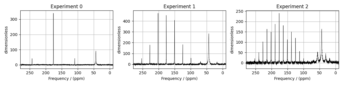
The following is a multi-dataset least-squares fitting example of \(^{13}\text{C}\) MAS NMR spectrum of Glycine spinning at 5 kHz, 1.94 kHz, and 960 Hz. Before trying multi-dataset fitting, we recommend that you first try individual fits. The experimental datasets are part of DMFIT [1] examples.
import csdmpy as cp
import numpy as np
import matplotlib.pyplot as plt
from lmfit import Minimizer

from mrsimulator import Simulator, SpinSystem, Site
from mrsimulator.method.lib import BlochDecaySpectrum
from mrsimulator import signal_processor as sp
from mrsimulator.utils import spectral_fitting as sf
from mrsimulator.utils import get_spectral_dimensions
from mrsimulator.spin_system.tensors import SymmetricTensor
Import the datasets
Import the datasets and assign the standard deviation of noise for each dataset. Here,
sigma1, sigma2, and sigma3 are the noise standard deviation for the
dataset acquired at 5 kHz, 1.94 kHz, and 960 Hz spinning speeds, respectively.
host = "https://nmr.cemhti.cnrs-orleans.fr/Dmfit/Help/csdm/"
filename1 = "13C MAS 5000Hz - Glycine.csdf"
filename2 = "13C MAS 1940Hz - Glycine.csdf"
filename3 = "13C MAS 960Hz - Glycine.csdf"

experiment1 = cp.load(host + filename1).real
experiment2 = cp.load(host + filename2).real
experiment3 = cp.load(host + filename3).real
experiments = [experiment1, experiment2, experiment3]

fig, ax = plt.subplots(1, 3, figsize=(12, 3), subplot_kw={"projection": "csdm"})
for i, experiment in enumerate(experiments):
    _ = [item.to("ppm", "nmr_frequency_ratio") for item in experiment.dimensions]

    # plot of the dataset.
    ax[i].plot(experiment, color="black", linewidth=0.5, label="Experiment")
    ax[i].set_title(f"Experiment {i}")
    ax[i].set_xlim(280, -10)
    ax[i].grid()
plt.tight_layout()
plt.show()
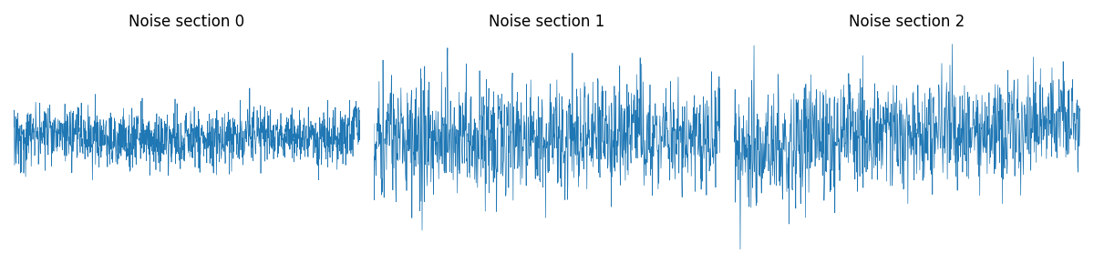
Estimate noise statistics from the dataset
noise_data = []
limits = [40e-6, 15e-6, 10e-6]
for measurement, cutoff in zip(experiments, limits):
    coords = measurement.dimensions[0].coordinates
    noise_region = np.where(coords < cutoff)
    noise_data.append(measurement[noise_region])

fig, ax = plt.subplots(
    1, 3, figsize=(12, 3), sharey=True, subplot_kw={"projection": "csdm"}
)
for i, noise in enumerate(noise_data):
    ax[i].plot(noise, linewidth=0.5, label="noise")
    ax[i].set_title(f"Noise section {i}")
    ax[i].axis("off")
plt.tight_layout()
plt.show()

noise_mean = [item.mean() for item in noise_data]
sigma = [item.std() for item in noise_data]
print("mean", noise_mean)
print("standard deviation", sigma)
mean [<Quantity 0.2857664>, <Quantity 0.2312411>, <Quantity 0.6193483>]
standard deviation [<Quantity 1.950852>, <Quantity 3.784959>, <Quantity 3.939941>]
Create a fitting model
Spin System: The objective of a multi-dataset fitting is to optimize the spin system parameters using multiple datasets. In this example, we create two single-site spin systems, which are then shared by three method objects.
C1 = Site(
    isotope="13C",
    isotropic_chemical_shift=176.0,  # in ppm
    shielding_symmetric=SymmetricTensor(zeta=60, eta=0.6),  # zeta in Hz
)
C2 = Site(
    isotope="13C",
    isotropic_chemical_shift=43.0,  # in ppm
    shielding_symmetric=SymmetricTensor(zeta=30, eta=0.5),  # zeta in Hz
)

spin_systems = [SpinSystem(sites=[C1], name="C1"), SpinSystem(sites=[C2], name="C2")]
Method: Create the three MAS method objects with respective MAS spinning speeds.
# Get the spectral dimension parameters from the respective experiment and setup the
# corresponding method.

# Method for dataset 1
spectral_dims1 = get_spectral_dimensions(experiment1)
MAS1 = BlochDecaySpectrum(
    channels=["13C"],
    magnetic_flux_density=7.05,  # in T
    rotor_frequency=5000,  # in Hz
    spectral_dimensions=spectral_dims1,
    experiment=experiment1,  # add experimental dataset 1
)

# Method for dataset 2
spectral_dims2 = get_spectral_dimensions(experiment2)
MAS2 = BlochDecaySpectrum(
    channels=["13C"],
    magnetic_flux_density=7.05,  # in T
    rotor_frequency=1940,  # in Hz
    spectral_dimensions=spectral_dims2,
    experiment=experiment2,  # add experimental dataset 2
)

# Method for dataset 3
spectral_dims3 = get_spectral_dimensions(experiment3)
MAS3 = BlochDecaySpectrum(
    channels=["13C"],
    magnetic_flux_density=7.05,  # in T
    rotor_frequency=960,  # in Hz
    spectral_dimensions=spectral_dims3,
    experiment=experiment3,  # add experimental dataset 3
)
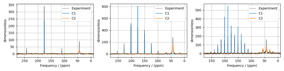
Guess Model Spectrum
# Simulation
# ----------
# Add the spin systems and the three methods to the simulator object.
sim = Simulator(spin_systems=spin_systems, methods=[MAS1, MAS2, MAS3])
sim.config.decompose_spectrum = "spin_system"
sim.run()

# Post Simulation Processing
# --------------------------
# Add signal processing to simulation dataset from the three methods.

# Processor for dataset 1
processor1 = sp.SignalProcessor(
    operations=[
        sp.IFFT(),
        sp.apodization.Exponential(FWHM="20 Hz", dv_index=0),  # spin system 0
        sp.apodization.Exponential(FWHM="200 Hz", dv_index=1),  # spin system 1
        sp.FFT(),
        sp.Scale(factor=100),  # dataset is scaled independently using scale factor.
    ]
)

# Processor for dataset 2
processor2 = sp.SignalProcessor(
    operations=[
        sp.IFFT(),
        sp.apodization.Exponential(FWHM="30 Hz", dv_index=0),  # spin system 0
        sp.apodization.Exponential(FWHM="300 Hz", dv_index=1),  # spin system 1
        sp.FFT(),
        sp.Scale(factor=1000),  # dataset is scaled independently using scale factor.
    ]
)

# Processor for dataset 3
processor3 = sp.SignalProcessor(
    operations=[
        sp.IFFT(),
        sp.apodization.Exponential(FWHM="10 Hz", dv_index=0),  # spin system 0
        sp.apodization.Exponential(FWHM="150 Hz", dv_index=1),  # spin system 1
        sp.FFT(),
        sp.Scale(factor=500),  # dataset is scaled independently using scale factor.
    ]
)
processors = [processor1, processor2, processor3]

processed_dataset = []
for i, proc in enumerate(processors):
    processed_dataset.append(
        proc.apply_operations(dataset=sim.methods[i].simulation).real
    )


# Plot of the guess Spectrum
# --------------------------

fig, ax = plt.subplots(1, 3, figsize=(12, 3), subplot_kw={"projection": "csdm"})
for i, exp_dataset in enumerate(experiments):
    ax[i].plot(exp_dataset, color="black", linewidth=0.5, label="Experiment")
    ax[i].plot(processed_dataset[i], linewidth=2, alpha=0.6)
    ax[i].set_xlim(280, -10)
    ax[i].grid()

plt.legend()
plt.tight_layout()
plt.show()
Least-squares minimization with LMFIT
Use the make_LMFIT_params() for a quick
setup of the fitting parameters. Note, the first two arguments of this function is
the simulator object and a list of SignalProcessor objects, processors. The
fitting parameters corresponding to the signal processor objects are generated using
SP_i_operation_j_FunctionName_FunctionArg, where i is the ith signal
processor within the list, j is the operation index of the ith processor, and
FunctionName and FunctionArg are the operation function name and function
argument, respectively.
params = sf.make_LMFIT_params(sim, processors, include={"rotor_frequency"})
print(params.pretty_print(columns=["value", "min", "max", "vary", "expr"]))
Name                                      Value      Min      Max     Vary     Expr
SP_0_operation_1_Exponential_FWHM            20     -inf      inf     True     None
SP_0_operation_2_Exponential_FWHM           200     -inf      inf     True     None
SP_0_operation_4_Scale_factor               100     -inf      inf     True     None
SP_1_operation_1_Exponential_FWHM            30     -inf      inf     True     None
SP_1_operation_2_Exponential_FWHM           300     -inf      inf     True     None
SP_1_operation_4_Scale_factor              1000     -inf      inf     True     None
SP_2_operation_1_Exponential_FWHM            10     -inf      inf     True     None
SP_2_operation_2_Exponential_FWHM           150     -inf      inf     True     None
SP_2_operation_4_Scale_factor               500     -inf      inf     True     None
mth_0_rotor_frequency                      5000     4900     5100     True     None
mth_1_rotor_frequency                      1940     1840     2040     True     None
mth_2_rotor_frequency                       960      860     1060     True     None
sys_0_abundance                              50        0      100     True     None
sys_0_site_0_isotropic_chemical_shift       176     -inf      inf     True     None
sys_0_site_0_shielding_symmetric_eta        0.6        0        1     True     None
sys_0_site_0_shielding_symmetric_zeta        60     -inf      inf     True     None
sys_1_abundance                              50        0      100    False 100-sys_0_abundance
sys_1_site_0_isotropic_chemical_shift        43     -inf      inf     True     None
sys_1_site_0_shielding_symmetric_eta        0.5        0        1     True     None
sys_1_site_0_shielding_symmetric_zeta        30     -inf      inf     True     None
None
Solve the minimizer using LMFIT
opt = sim.optimize()  # Pre-compute transition pathways
minner = Minimizer(
    sf.LMFIT_min_function,
    params,
    fcn_args=(sim, processors, sigma),
    fcn_kws={"opt": opt},
)
result = minner.minimize()
result
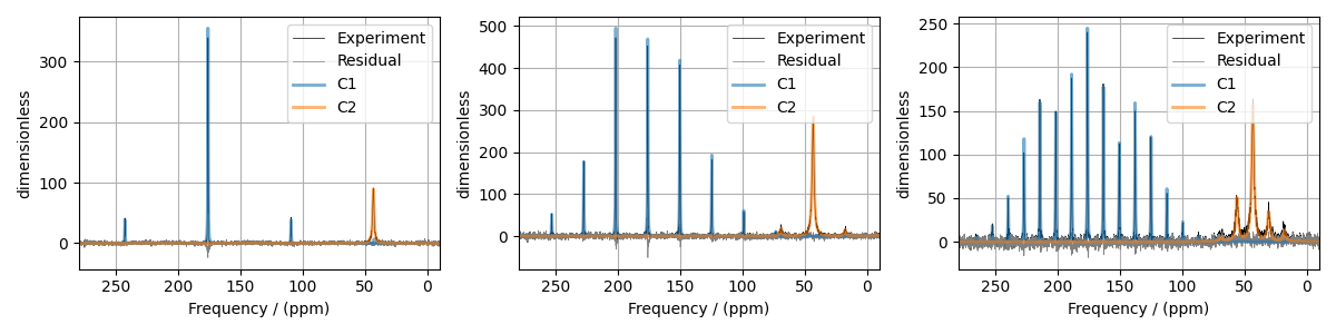
The best fit solution
all_best_fit = sf.bestfit(sim, processors)  # a list of best fit simulations
all_residuals = sf.residuals(sim, processors)  # a list of residuals

# Plot the spectrum
fig, ax = plt.subplots(1, 3, figsize=(12, 3), subplot_kw={"projection": "csdm"})
for i, proc in enumerate(processors):
    ax[i].plot(experiments[i], color="black", linewidth=0.5, label="Experiment")
    ax[i].plot(all_residuals[i].real, color="gray", linewidth=0.5, label="Residual")
    ax[i].plot(all_best_fit[i].real, linewidth=2, alpha=0.6)
    ax[i].set_xlim(280, -10)
    ax[i].grid()

plt.legend()
plt.tight_layout()
plt.show()
Total running time of the script: (0 minutes 8.721 seconds)