Note
Go to the end to download the full example code.
¹⁷O MAS NMR of crystalline Na₂SiO₃ (2nd order quad)
In this example, we illustrate the use of the mrsimulator objects to
create a quadrupolar fitting model using Simulator and SignalProcessor objects,
use the fitting model to perform a least-squares analysis, and
extract the fitting parameters from the model.
We use the LMFIT library to fit the spectrum. The following example shows the least-squares fitting procedure applied to the \(^{17}\text{O}\) MAS NMR spectrum of \(\text{Na}_{2}\text{SiO}_{3}\) [1].
Start by importing the relevant modules.
import csdmpy as cp
import numpy as np
import matplotlib.pyplot as plt
from lmfit import Minimizer

from mrsimulator import Simulator, SpinSystem, Site
from mrsimulator.method.lib import BlochDecayCTSpectrum
from mrsimulator import signal_processor as sp
from mrsimulator.utils import spectral_fitting as sf
from mrsimulator.utils import get_spectral_dimensions
from mrsimulator.spin_system.tensors import SymmetricTensor
Import the dataset
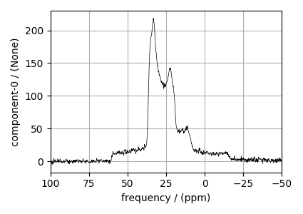
Import the experimental dataset. We use dataset file serialized with the CSDM file-format, using the csdmpy module.
filename = "https://ssnmr.org/sites/default/files/mrsimulator/Na2SiO3_O17.csdf"
experiment = cp.load(filename)

# For spectral fitting, we only focus on the real part of the complex dataset
experiment = experiment.real

# Convert the dimension coordinates from Hz to ppm.
experiment.x[0].to("ppm", "nmr_frequency_ratio")

# plot of the dataset.
plt.figure(figsize=(4.25, 3.0))
ax = plt.subplot(projection="csdm")
ax.plot(experiment, color="black", linewidth=0.5, label="Experiment")
ax.set_xlim(100, -50)
plt.grid()
plt.tight_layout()
plt.show()
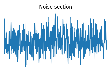
Estimate noise statistics from the dataset
coords = experiment.dimensions[0].coordinates
noise_region = np.where(coords > 70e-6)
noise_data = experiment[noise_region]

plt.figure(figsize=(3.75, 2.5))
ax = plt.subplot(projection="csdm")
ax.plot(noise_data, label="noise")
plt.title("Noise section")
plt.axis("off")
plt.tight_layout()
plt.show()

noise_mean, sigma = experiment[noise_region].mean(), experiment[noise_region].std()
noise_mean, sigma
(<Quantity 0.13096036>, <Quantity 1.710335>)
Create a fitting model
A fitting model is a composite of Simulator and SignalProcessor objects.
Step 1: Create initial guess sites and spin systems
O1 = Site(
    isotope="17O",
    isotropic_chemical_shift=60.0,  # in ppm,
    quadrupolar=SymmetricTensor(Cq=4.2e6, eta=0.5),  # Cq in Hz
)

O2 = Site(
    isotope="17O",
    isotropic_chemical_shift=40.0,  # in ppm,
    quadrupolar=SymmetricTensor(Cq=2.4e6, eta=0.0),  # Cq in Hz
)

spin_systems = [
    SpinSystem(sites=[O1], abundance=50, name="O1"),
    SpinSystem(sites=[O2], abundance=50, name="O2"),
]
Step 2: Create the method object. Create an appropriate method object that closely resembles the technique used in acquiring the experimental dataset. The attribute values of this method must meet the experimental conditions, including the acquisition channels, the magnetic flux density, rotor angle, rotor frequency, and the spectral/spectroscopic dimension.
In the following example, we set up a central transition selective Bloch decay
spectrum method where the spectral/spectroscopic dimension information, i.e., count,
spectral_width, and the reference_offset, is extracted from the CSDM dimension
metadata using the get_spectral_dimensions() utility
function. The remaining attribute values are set to the experimental conditions.
# get the count, spectral_width, and reference_offset information from the experiment.
spectral_dims = get_spectral_dimensions(experiment)

MAS_CT = BlochDecayCTSpectrum(
    channels=["17O"],
    magnetic_flux_density=9.395,  # in T
    rotor_frequency=14000,  # in Hz
    spectral_dimensions=spectral_dims,
    experiment=experiment,  # experimental dataset
)
Step 3: Create the Simulator object and add the method and spin system objects.
Step 4: Create a SignalProcessor class object and apply the post-simulation signal processor operations.
processor = sp.SignalProcessor(
    operations=[
        sp.IFFT(),
        sp.apodization.Gaussian(FWHM="100 Hz"),
        sp.FFT(),
        sp.Scale(factor=2000.0),
    ]
)
processed_dataset = processor.apply_operations(dataset=sim.methods[0].simulation).real
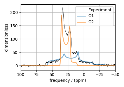
Step 5: The plot of the dataset and the guess spectrum.
plt.figure(figsize=(4.25, 3.0))
ax = plt.subplot(projection="csdm")
ax.plot(experiment, color="black", linewidth=0.5, label="Experiment")
ax.plot(processed_dataset, linewidth=2, alpha=0.6)
ax.set_xlim(100, -50)
plt.legend()
plt.grid()
plt.tight_layout()
plt.show()
Least-squares minimization with LMFIT
Once you have a fitting model, you need to create the list of parameters to use in the
least-squares fitting. For this, you may use the
Parameters class from LMFIT,
as described in the previous example.
Here, we make use of a utility function,
make_LMFIT_params(), that considerably
simplifies the LMFIT parameters generation process.
Step 6: Create a list of parameters.
params = sf.make_LMFIT_params(sim, processor)
The make_LMFIT_params parses the instances of the Simulator and the
PostSimulator objects for parameters and returns a LMFIT Parameters object.
Customize the Parameters:
You may customize the parameters list, params, as desired. Here, we remove the
abundance of the two spin systems and constrain it to the initial value of 50% each,
and constrain eta=0 for spin system at index 1.
params.pop("sys_0_abundance")
params.pop("sys_1_abundance")
params["sys_1_site_0_quadrupolar_eta"].vary = False
print(params.pretty_print(columns=["value", "min", "max", "vary", "expr"]))
Name                                      Value      Min      Max     Vary     Expr
SP_0_operation_1_Gaussian_FWHM              100     -inf      inf     True     None
SP_0_operation_3_Scale_factor              2000     -inf      inf     True     None
sys_0_site_0_isotropic_chemical_shift        60     -inf      inf     True     None
sys_0_site_0_quadrupolar_Cq             4.2e+06     -inf      inf     True     None
sys_0_site_0_quadrupolar_eta                0.5        0        1     True     None
sys_1_site_0_isotropic_chemical_shift        40     -inf      inf     True     None
sys_1_site_0_quadrupolar_Cq             2.4e+06     -inf      inf     True     None
sys_1_site_0_quadrupolar_eta                  0        0        1    False     None
None
Step 7: Perform least-squares minimization. For the user’s convenience, we also
provide a utility function,
LMFIT_min_function(), for evaluating the
difference vector between the simulation and experiment, based on
the parameters update. You may use this function directly to instantiate the
LMFIT Minimizer class where fcn_args and fcn_kws are arguments passed to the
function, as follows,
opt = sim.optimize()
minner = Minimizer(
    sf.LMFIT_min_function,
    params,
    fcn_args=(sim, processor, sigma),
    fcn_kws={"opt": opt},
)
result = minner.minimize()
result
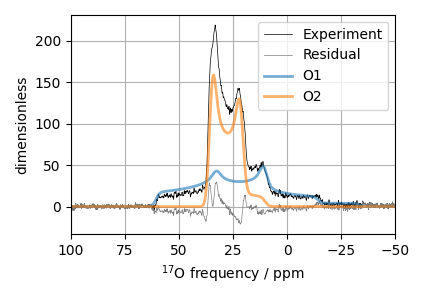
Step 8: The plot of the fit and the measurement dataset.
# Best fit spectrum
best_fit = sf.bestfit(sim, processor)[0].real
residuals = sf.residuals(sim, processor)[0].real

plt.figure(figsize=(4.25, 3.0))
ax = plt.subplot(projection="csdm")
ax.plot(experiment, color="black", linewidth=0.5, label="Experiment")
ax.plot(residuals, color="gray", linewidth=0.5, label="Residual")
ax.plot(best_fit, linewidth=2, alpha=0.6)
ax.set_xlabel("$^{17}$O frequency / ppm")
ax.set_xlim(100, -50)
plt.legend()
plt.grid()
plt.tight_layout()
plt.show()
Total running time of the script: (0 minutes 3.214 seconds)