Note
Go to the end to download the full example code.
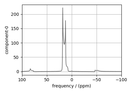
¹¹B MAS NMR of Lithium orthoborate crystal
The following is a quadrupolar lineshape fitting example for the 11B MAS NMR of lithium orthoborate crystal. The dataset was shared by Dr. Nathan Barrow.
import csdmpy as cp
import numpy as np
import matplotlib.pyplot as plt
from lmfit import Minimizer

from mrsimulator import Simulator, Site, SpinSystem
from mrsimulator.method.lib import BlochDecayCTSpectrum
from mrsimulator import signal_processor as sp
from mrsimulator.utils import spectral_fitting as sf
from mrsimulator.utils import get_spectral_dimensions
from mrsimulator.spin_system.tensors import SymmetricTensor
Import the dataset
host = "https://ssnmr.org/sites/default/files/mrsimulator/"
filename = "11B_lithum_orthoborate.csdf"
experiment = cp.load(host + filename)

# For spectral fitting, we only focus on the real part of the complex dataset
experiment = experiment.real

# Convert the coordinates along each dimension from Hz to ppm.
_ = [item.to("ppm", "nmr_frequency_ratio") for item in experiment.dimensions]

# plot of the dataset.
plt.figure(figsize=(4.25, 3.0))
ax = plt.subplot(projection="csdm")
ax.plot(experiment, "k", alpha=0.5)
ax.set_xlim(100, -100)
plt.grid()
plt.tight_layout()
plt.show()
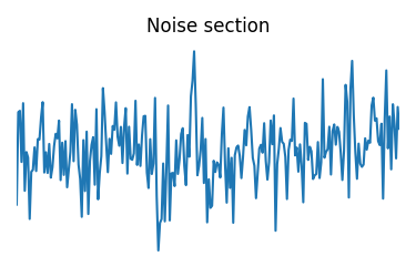
Estimate noise statistics from the dataset
coords = experiment.dimensions[0].coordinates
noise_region = np.where(np.logical_and(coords < -140e-6, coords > -200e-6))
noise_data = experiment[noise_region]

plt.figure(figsize=(3.75, 2.5))
ax = plt.subplot(projection="csdm")
ax.plot(noise_data, label="noise")
plt.title("Noise section")
plt.axis("off")
plt.tight_layout()
plt.show()

noise_mean, sigma = experiment[noise_region].mean(), experiment[noise_region].std()
noise_mean, sigma
(<Quantity 0.12421671>, <Quantity 0.07768127>)
Create a fitting model
Spin System
B11 = Site(
    isotope="11B",
    isotropic_chemical_shift=20.0,  # in ppm
    quadrupolar=SymmetricTensor(Cq=2.3e6, eta=0.03),  # Cq in Hz
)
spin_systems = [SpinSystem(sites=[B11])]
Method
# Get the spectral dimension parameters from the experiment.
spectral_dims = get_spectral_dimensions(experiment)

MAS_CT = BlochDecayCTSpectrum(
    channels=["11B"],
    magnetic_flux_density=14.1,  # in T
    rotor_frequency=12500,  # in Hz
    spectral_dimensions=spectral_dims,
    experiment=experiment,  # add the measurement to the method.
)
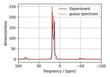
Guess Model Spectrum
# Simulation
# ----------
sim = Simulator(spin_systems=spin_systems, methods=[MAS_CT])
sim.run()

# Post Simulation Processing
# --------------------------
processor = sp.SignalProcessor(
    operations=[
        sp.IFFT(),
        sp.apodization.Exponential(FWHM="100 Hz"),
        sp.FFT(),
        sp.Scale(factor=2000),
    ]
)
processed_dataset = processor.apply_operations(dataset=sim.methods[0].simulation).real

# Plot of the guess Spectrum
# --------------------------
plt.figure(figsize=(4.25, 3.0))
ax = plt.subplot(projection="csdm")
ax.plot(experiment, "k", linewidth=1, label="Experiment")
ax.plot(processed_dataset, "r", alpha=0.75, linewidth=1, label="guess spectrum")
ax.set_xlim(100, -100)
plt.grid()
plt.legend()
plt.tight_layout()
plt.show()
Least-squares minimization with LMFIT
Use the make_LMFIT_params() for a quick
setup of the fitting parameters.
params = sf.make_LMFIT_params(sim, processor)
params.pop("sys_0_abundance")
print(params.pretty_print(columns=["value", "min", "max", "vary", "expr"]))
Name                                      Value      Min      Max     Vary     Expr
SP_0_operation_1_Exponential_FWHM           100     -inf      inf     True     None
SP_0_operation_3_Scale_factor              2000     -inf      inf     True     None
sys_0_site_0_isotropic_chemical_shift        20     -inf      inf     True     None
sys_0_site_0_quadrupolar_Cq             2.3e+06     -inf      inf     True     None
sys_0_site_0_quadrupolar_eta               0.03        0        1     True     None
None
Solve the minimizer using LMFIT
opt = sim.optimize()  # Pre-compute transition pathways
minner = Minimizer(
    sf.LMFIT_min_function,
    params,
    fcn_args=(sim, processor, sigma),
    fcn_kws={"opt": opt},
)
result = minner.minimize()
result
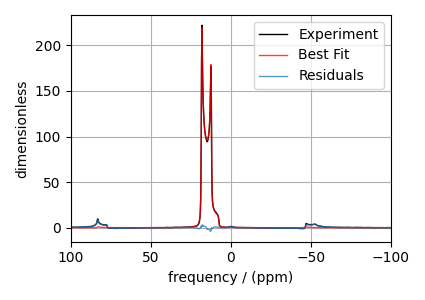
The best fit solution
best_fit = sf.bestfit(sim, processor)[0].real
residuals = sf.residuals(sim, processor)[0].real

# Plot the spectrum
plt.figure(figsize=(4.25, 3.0))
ax = plt.subplot(projection="csdm")
ax.plot(experiment, "k", linewidth=1, label="Experiment")
ax.plot(best_fit, "r", alpha=0.75, linewidth=1, label="Best Fit")
ax.plot(residuals, alpha=0.75, linewidth=1, label="Residuals")
ax.set_xlim(100, -100)
plt.grid()
plt.legend()
plt.tight_layout()
plt.show()
Total running time of the script: (0 minutes 1.920 seconds)