Note
Go to the end to download the full example code.
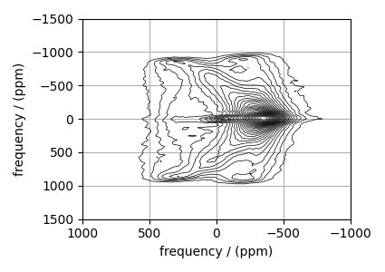
NiCl₂.2D₂O, ²H (I=1) Shifting-d echo
²H (I=1) 2D NMR CSA-Quad 1st order correlation spectrum.
The following is an example of fitting static shifting-d echo NMR correlation spectrum of \(\text{NiCl}_2\cdot 2\text{D}_2\text{O}\) crystalline solid. The spectrum used here is from Walder et al. [1].
import numpy as np
import csdmpy as cp
import matplotlib.pyplot as plt
from lmfit import Minimizer

from mrsimulator import Simulator, Site, SpinSystem
from mrsimulator import signal_processor as sp
from mrsimulator.utils import spectral_fitting as sf
from mrsimulator.utils import get_spectral_dimensions
from mrsimulator.spin_system.tensors import SymmetricTensor
from mrsimulator.method import Method, SpectralDimension, SpectralEvent, RotationEvent
Import the dataset
filename = "https://ssnmr.org/sites/default/files/mrsimulator/NiCl2.2D2O.csdf"
experiment = cp.load(filename)

# For spectral fitting, we only focus on the real part of the complex dataset
experiment = experiment.real

# Convert the coordinates along each dimension from Hz to ppm.
_ = [item.to("ppm", "nmr_frequency_ratio") for item in experiment.dimensions]

# plot of the dataset.
max_amp = experiment.max()
levels = (np.arange(29) + 1) * max_amp / 30  # contours are drawn at these levels.
options = dict(levels=levels, linewidths=0.5)  # plot options

plt.figure(figsize=(4.25, 3.0))
ax = plt.subplot(projection="csdm")
ax.contour(experiment, colors="k", **options)
ax.set_xlim(1000, -1000)
ax.set_ylim(1500, -1500)
plt.grid()
plt.tight_layout()
plt.show()
Estimate noise statistics from the dataset
coords = experiment.dimensions[0].coordinates
noise_region = np.where(coords > 700e-6)
noise_data = experiment[noise_region]

plt.figure(figsize=(3.75, 2.5))
ax = plt.subplot(projection="csdm")
ax.imshow(noise_data, aspect="auto", interpolation="none")
plt.title("Noise section")
plt.axis("off")
plt.tight_layout()
plt.show()

noise_mean, sigma = experiment[noise_region].mean(), experiment[noise_region].std()
noise_mean, sigma
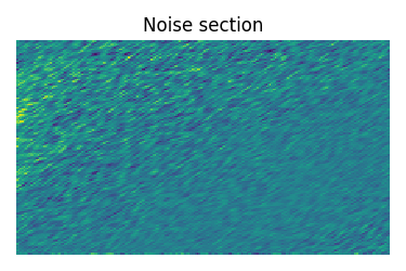
(<Quantity 0.64582>, <Quantity 5.835975>)
Create a fitting model
Guess model
Create a guess list of spin systems.
site = Site(
    isotope="2H",
    isotropic_chemical_shift=-90,  # in ppm
    shielding_symmetric=SymmetricTensor(
        zeta=-610,  # in ppm
        eta=0.15,
        alpha=0.7,  # in rads
        beta=2.0,  # in rads
        gamma=3.0,  # in rads
    ),
    quadrupolar=SymmetricTensor(Cq=75.2e3, eta=0.9),  # Cq in Hz
)

spin_systems = [SpinSystem(sites=[site])]
Method
Use the generic method, Method, to generate a shifting-d echo method. The
reported shifting-d 2D sequence is a correlation of the shielding frequencies to the
first-order quadrupolar frequencies. Here, we create a correlation method using the
freq_contrib attribute, which acts as a switch
for including the frequency contributions from interaction during the event.
In the following method, we assign the ["Quad1_2"] and
["Shielding1_0", "Shielding1_2"] as the value to the freq_contrib key. The
Quad1_2 is an enumeration for selecting the first-order second-rank quadrupolar
frequency contributions. Shielding1_0 and Shielding1_2 are enumerations for
the first-order shielding with zeroth and second-rank tensor contributions,
respectively. See FrequencyEnum for details.
# Get the spectral dimension parameters from the experiment.
spectral_dims = get_spectral_dimensions(experiment)

shifting_d = Method(
    channels=["2H"],
    magnetic_flux_density=9.395,  # in T
    rotor_frequency=0,  # in Hz
    rotor_angle=0,  # in rads
    spectral_dimensions=[
        SpectralDimension(
            **spectral_dims[0],
            label="Quadrupolar frequency",
            events=[
                SpectralEvent(
                    transition_queries=[{"ch1": {"P": [-1]}}],
                    freq_contrib=["Quad1_2"],
                ),
                RotationEvent(),
            ],
        ),
        SpectralDimension(
            **spectral_dims[1],
            label="Paramagnetic shift",
            events=[
                SpectralEvent(
                    transition_queries=[{"ch1": {"P": [-1]}}],
                    freq_contrib=["Shielding1_0", "Shielding1_2"],
                )
            ],
        ),
    ],
    experiment=experiment,  # also add the measurement to the method.
)
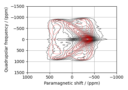
Guess Spectrum
# Simulation
# ----------
sim = Simulator(spin_systems=spin_systems, methods=[shifting_d])
sim.config.integration_volume = "hemisphere"
sim.run()

# Post Simulation Processing
# --------------------------
processor = sp.SignalProcessor(
    operations=[
        # Gaussian convolution along both dimensions.
        sp.IFFT(dim_index=(0, 1)),
        sp.apodization.Gaussian(FWHM="5 kHz", dim_index=0),  # along dimension 0
        sp.apodization.Gaussian(FWHM="5 kHz", dim_index=1),  # along dimension 1
        sp.FFT(dim_index=(0, 1)),
        sp.Scale(factor=5e9),
    ]
)
processed_dataset = processor.apply_operations(dataset=sim.methods[0].simulation).real

# Plot of the guess Spectrum
# --------------------------
plt.figure(figsize=(4.25, 3.0))
ax = plt.subplot(projection="csdm")
ax.contour(experiment, colors="k", **options)
ax.contour(processed_dataset, colors="r", linestyles="--", **options)
ax.set_xlim(1000, -1000)
ax.set_ylim(1500, -1500)
plt.grid()
plt.tight_layout()
plt.show()
Least-squares minimization with LMFIT
Use the make_LMFIT_params() for a quick
setup of the fitting parameters.
params = sf.make_LMFIT_params(sim, processor)
print(params.pretty_print(columns=["value", "min", "max", "vary", "expr"]))
Name                                       Value      Min      Max     Vary     Expr
SP_0_operation_1_Gaussian_FWHM                 5     -inf      inf     True     None
SP_0_operation_2_Gaussian_FWHM                 5     -inf      inf     True     None
SP_0_operation_4_Scale_factor              5e+09     -inf      inf     True     None
sys_0_abundance                              100        0      100    False      100
sys_0_site_0_isotropic_chemical_shift        -90     -inf      inf     True     None
sys_0_site_0_quadrupolar_Cq             7.52e+04     -inf      inf     True     None
sys_0_site_0_quadrupolar_eta                 0.9        0        1     True     None
sys_0_site_0_shielding_symmetric_alpha       0.7     -inf      inf     True     None
sys_0_site_0_shielding_symmetric_beta          2     -inf      inf     True     None
sys_0_site_0_shielding_symmetric_eta        0.15        0        1     True     None
sys_0_site_0_shielding_symmetric_gamma         3     -inf      inf     True     None
sys_0_site_0_shielding_symmetric_zeta       -610     -inf      inf     True     None
None
Solve the minimizer using LMFIT
opt = sim.optimize()  # Pre-compute transition pathways
minner = Minimizer(
    sf.LMFIT_min_function,
    params,
    fcn_args=(sim, processor, sigma),
    fcn_kws={"opt": opt},
)
result = minner.minimize()
result
The best fit solution
best_fit = sf.bestfit(sim, processor)[0].real

# Plot the spectrum
plt.figure(figsize=(4.25, 3.0))
ax = plt.subplot(projection="csdm")
ax.contour(experiment, colors="k", **options)
ax.contour(best_fit, colors="r", linestyles="--", **options)
ax.set_xlim(1000, -1000)
ax.set_ylim(1500, -1500)
plt.grid()
plt.tight_layout()
plt.show()
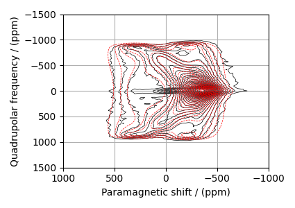
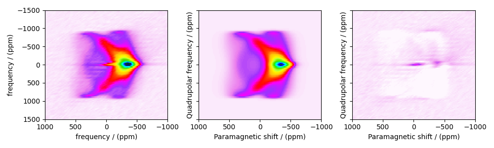
Image plots with residuals
residuals = sf.residuals(sim, processor)[0].real

fig, ax = plt.subplots(
    1, 3, sharey=True, figsize=(10, 3.0), subplot_kw={"projection": "csdm"}
)
vmax, vmin = experiment.max(), experiment.min()
for i, dat in enumerate([experiment, best_fit, residuals]):
    ax[i].imshow(
        dat,
        aspect="auto",
        cmap="gist_ncar_r",
        vmax=vmax,
        vmin=vmin,
        interpolation="none",
    )
    ax[i].set_xlim(1000, -1000)
ax[0].set_ylim(1500, -1500)
plt.tight_layout()
plt.show()
Total running time of the script: (0 minutes 4.197 seconds)