Note
Go to the end to download the full example code.
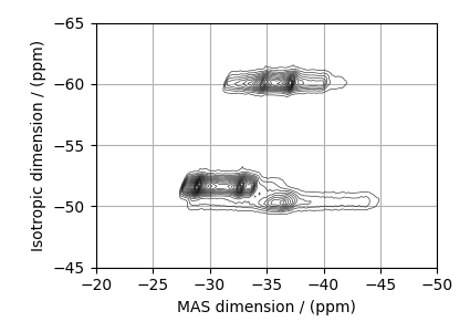
⁸⁷Rb 2D 3QMAS NMR of RbNO₃
The following is a 3QMAS fitting example for \(\text{RbNO}_3\). The dataset was acquired and shared by Brendan Wilson.
import numpy as np
import csdmpy as cp
import matplotlib.pyplot as plt
from lmfit import Minimizer

from mrsimulator import Simulator
from mrsimulator.method.lib import ThreeQ_VAS
from mrsimulator import signal_processor as sp
from mrsimulator.utils import spectral_fitting as sf
from mrsimulator.utils import get_spectral_dimensions
from mrsimulator.utils.collection import single_site_system_generator
Import the dataset
filename = "https://ssnmr.org/sites/default/files/mrsimulator/RbNO3_MQMAS.csdf"
experiment = cp.load(filename)

# For spectral fitting, we only focus on the real part of the complex dataset
experiment = experiment.real

# Convert the coordinates along each dimension from Hz to ppm.
_ = [item.to("ppm", "nmr_frequency_ratio") for item in experiment.dimensions]

# plot of the dataset.
max_amp = experiment.max()
levels = (np.arange(24) + 1) * max_amp / 25  # contours are drawn at these levels.
options = dict(levels=levels, alpha=0.75, linewidths=0.5)  # plot options

plt.figure(figsize=(4.25, 3.0))
ax = plt.subplot(projection="csdm")
ax.contour(experiment, colors="k", **options)
ax.set_xlim(-20, -50)
ax.set_ylim(-45, -65)
plt.grid()
plt.tight_layout()
plt.show()
Estimate noise statistics from the dataset.
noise_region = np.where(experiment.dimensions[0].coordinates > -25e-6)
noise_data = experiment[noise_region]

plt.figure(figsize=(3.75, 2.5))
ax = plt.subplot(projection="csdm")
ax.imshow(noise_data, aspect="auto", interpolation="none")
plt.title("Noise section")
plt.axis("off")
plt.tight_layout()
plt.show()

noise_mean, sigma = noise_data.mean(), noise_data.std()
noise_mean, sigma
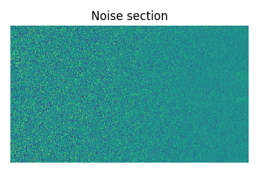
(<Quantity 1.1995176>, <Quantity 159.38718>)
Create a fitting model
Guess model
Create a guess list of spin systems.
shifts = [-26.8, -28.4, -31.2]  # in ppm
Cq = [1.7e6, 2.0e6, 1.7e6]  # in  Hz
eta = [0.2, 0.95, 0.6]
abundance = [40.0, 25.0, 35.0]  # in %

spin_systems = single_site_system_generator(
    isotope="87Rb",
    isotropic_chemical_shift=shifts,
    quadrupolar={"Cq": Cq, "eta": eta},
    abundance=abundance,
)
Method
Create the 3QMAS method.
# Get the spectral dimension parameters from the experiment.
spectral_dims = get_spectral_dimensions(experiment)

MQMAS = ThreeQ_VAS(
    channels=["87Rb"],
    magnetic_flux_density=9.395,  # in T
    spectral_dimensions=spectral_dims,
    experiment=experiment,  # add the measurement to the method.
)
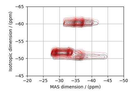
Guess Spectrum
# Simulation
# ----------
sim = Simulator(spin_systems=spin_systems, methods=[MQMAS])
sim.config.number_of_sidebands = 1
sim.run()

# Post Simulation Processing
# --------------------------
processor = sp.SignalProcessor(
    operations=[
        # Gaussian convolution along both dimensions.
        sp.IFFT(dim_index=(0, 1)),
        sp.apodization.Gaussian(FWHM="0.08 kHz", dim_index=0),
        sp.apodization.Gaussian(FWHM="0.2 kHz", dim_index=1),
        sp.FFT(dim_index=(0, 1)),
        sp.Scale(factor=2e8),
    ]
)
processed_dataset = processor.apply_operations(dataset=sim.methods[0].simulation).real

# Plot of the guess Spectrum
# --------------------------
plt.figure(figsize=(4.25, 3.0))
ax = plt.subplot(projection="csdm")
ax.contour(experiment, colors="k", **options)
ax.contour(processed_dataset, colors="r", linestyles="--", **options)
ax.set_xlim(-20, -50)
ax.set_ylim(-45, -65)
plt.grid()
plt.tight_layout()
plt.show()
Least-squares minimization with LMFIT
Use the make_LMFIT_params() for a quick
setup of the fitting parameters.
params = sf.make_LMFIT_params(sim, processor)
print(params.pretty_print(columns=["value", "min", "max", "vary", "expr"]))
Name                                      Value      Min      Max     Vary     Expr
SP_0_operation_1_Gaussian_FWHM             0.08     -inf      inf     True     None
SP_0_operation_2_Gaussian_FWHM              0.2     -inf      inf     True     None
SP_0_operation_4_Scale_factor             2e+08     -inf      inf     True     None
sys_0_abundance                              40        0      100     True     None
sys_0_site_0_isotropic_chemical_shift     -26.8     -inf      inf     True     None
sys_0_site_0_quadrupolar_Cq             1.7e+06     -inf      inf     True     None
sys_0_site_0_quadrupolar_eta                0.2        0        1     True     None
sys_1_abundance                              25        0      100     True     None
sys_1_site_0_isotropic_chemical_shift     -28.4     -inf      inf     True     None
sys_1_site_0_quadrupolar_Cq               2e+06     -inf      inf     True     None
sys_1_site_0_quadrupolar_eta               0.95        0        1     True     None
sys_2_abundance                              35        0      100    False 100-sys_0_abundance-sys_1_abundance
sys_2_site_0_isotropic_chemical_shift     -31.2     -inf      inf     True     None
sys_2_site_0_quadrupolar_Cq             1.7e+06     -inf      inf     True     None
sys_2_site_0_quadrupolar_eta                0.6        0        1     True     None
None
Solve the minimizer using LMFIT
opt = sim.optimize()  # Pre-compute transition pathways
minner = Minimizer(
    sf.LMFIT_min_function,
    params,
    fcn_args=(sim, processor, sigma),
    fcn_kws={"opt": opt},
)
result = minner.minimize()
result
The best fit solution
best_fit = sf.bestfit(sim, processor)[0].real

# Plot the spectrum
plt.figure(figsize=(4.25, 3.0))
ax = plt.subplot(projection="csdm")
ax.contour(experiment, colors="k", **options)
ax.contour(best_fit, colors="r", linestyles="--", **options)
ax.set_xlim(-20, -50)
ax.set_ylim(-45, -65)
plt.grid()
plt.tight_layout()
plt.show()
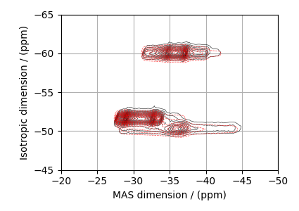
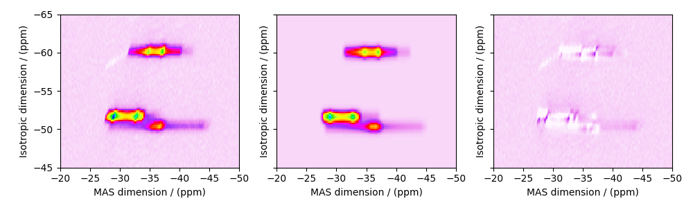
Image plots with residuals
residuals = sf.residuals(sim, processor)[0].real

fig, ax = plt.subplots(
    1, 3, sharey=True, figsize=(10, 3.0), subplot_kw={"projection": "csdm"}
)
vmax, vmin = experiment.max(), experiment.min()
for i, dat in enumerate([experiment, best_fit, residuals]):
    ax[i].imshow(
        dat,
        aspect="auto",
        cmap="gist_ncar_r",
        vmax=vmax,
        vmin=vmin,
        interpolation="none",
    )
    ax[i].set_xlim(-20, -50)
ax[0].set_ylim(-45, -65)
plt.tight_layout()
plt.show()
Total running time of the script: (0 minutes 6.041 seconds)