Rb₂CrO₄, ⁸⁷Rb (I=3/2) SAS¶

⁸⁷Rb (I=3/2) Switched-angle spinning (SAS) simulation.

The following is a Switched-Angle Spinning (SAS) simulation of \(\text{Rb}_2\text{CrO}_4\). While \(\text{Rb}_2\text{CrO}_4\) has two rubidium sites, the site with the smaller quadrupolar interaction was selectively observed and reported by Shore et al. [1]. The following is the simulation based on the published tensor parameters.

import matplotlib.pyplot as plt
import numpy as np

from mrsimulator import Simulator, SpinSystem, Site
from mrsimulator.method import Method, SpectralDimension, SpectralEvent
from mrsimulator import signal_processor as sp
from mrsimulator.spin_system.tensors import SymmetricTensor

Generate the site and spin system objects.

site = Site(
    isotope="87Rb",
    isotropic_chemical_shift=-7,  # in ppm
    shielding_symmetric=SymmetricTensor(zeta=110, eta=0),
    quadrupolar=SymmetricTensor(
        Cq=3.5e6,  # in Hz
        eta=0.3,
        alpha=0,  # in rads
        beta=70 * 3.14159 / 180,  # in rads
        gamma=0,  # in rads
    ),
)
spin_system = SpinSystem(sites=[site])

Use the generic method, Method, to simulate a 2D SAS spectrum by customizing the method parameters, as shown below.

sas = Method(
    channels=["87Rb"],
    magnetic_flux_density=4.2,  # in T
    rotor_frequency=np.inf,
    spectral_dimensions=[
        SpectralDimension(
            count=256,
            spectral_width=1.5e4,  # in Hz
            reference_offset=-5e3,  # in Hz
            label="70.12 dimension",
            events=[
                SpectralEvent(
                    rotor_angle=70.12 * 3.14159 / 180,  # in radians
                    transition_queries=[{"ch1": {"P": [-1], "D": [0]}}],
                )
            ],
        ),
        SpectralDimension(
            count=512,
            spectral_width=15e3,  # in Hz
            reference_offset=-7e3,  # in Hz
            label="MAS dimension",
            events=[
                SpectralEvent(
                    rotor_angle=54.74 * 3.14159 / 180,  # in radians
                    transition_queries=[{"ch1": {"P": [-1], "D": [0]}}],
                )
            ],
        ),
    ],
)

Create the Simulator object, add the method and spin system objects, and run the simulation.

sim = Simulator()
sim.spin_systems = [spin_system]  # add the spin systems
sim.methods = [sas]  # add the method.

# Configure the simulator object. For non-coincidental tensors, set the value of the
# `integration_volume` attribute to `hemisphere`.
sim.config.integration_volume = "hemisphere"
sim.run()

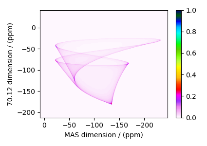
The plot of the simulation.

dataset = sim.methods[0].simulation

plt.figure(figsize=(4.25, 3.0))
ax = plt.subplot(projection="csdm")
cb = ax.imshow(dataset.real / dataset.real.max(), aspect="auto", cmap="gist_ncar_r")
plt.colorbar(cb)
ax.invert_xaxis()
plt.tight_layout()
plt.show()

Add post-simulation signal processing.

processor = sp.SignalProcessor(
    operations=[
        # Gaussian convolution along both dimensions.
        sp.IFFT(dim_index=(0, 1)),
        sp.apodization.Gaussian(FWHM="0.2 kHz", dim_index=0),
        sp.apodization.Gaussian(FWHM="0.2 kHz", dim_index=1),
        sp.FFT(dim_index=(0, 1)),
    ]
)
processed_dataset = processor.apply_operations(dataset=dataset)
processed_dataset /= processed_dataset.max()

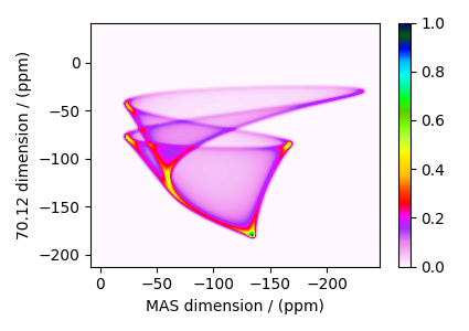
The plot of the simulation after signal processing.

plt.figure(figsize=(4.25, 3.0))
ax = plt.subplot(projection="csdm")
cb = ax.imshow(processed_dataset.real, cmap="gist_ncar_r", aspect="auto")
plt.colorbar(cb)
ax.invert_xaxis()
plt.tight_layout()
plt.show()

Total running time of the script: ( 0 minutes 0.825 seconds)

Gallery generated by Sphinx-Gallery