Coesite, ¹⁷O (I=5/2) 3QMAS¶

¹⁷O (I=5/2) 3QMAS simulation.

The following is a triple quantum magic angle spinning (3QMAS) simulation of Coesite. The NMR EFG tensor parameters for \(^{17}\text{O}\) sites in coesite is obtained from Grandinetti et al. [1]

import matplotlib.pyplot as plt

from mrsimulator import Simulator
from mrsimulator.method.lib import ThreeQ_VAS
from mrsimulator import signal_processor as sp
from mrsimulator.method import SpectralDimension

Create the Simulator object and load the spin systems database or url address.

sim = Simulator()

# load the spin systems from url.
filename = "https://ssnmr.org/sites/default/files/mrsimulator/coesite_0.mrsys"
sim.load_spin_systems(filename)

method = ThreeQ_VAS(
    channels=["17O"],
    magnetic_flux_density=11.74,  # in T
    spectral_dimensions=[
        SpectralDimension(
            count=256,
            spectral_width=5e3,  # in Hz
            reference_offset=-2.5e3,  # in Hz
            label="Isotropic dimension",
        ),
        # The last spectral dimension block is the direct-dimension
        SpectralDimension(
            count=256,
            spectral_width=2e4,  # in Hz
            reference_offset=0,  # in Hz
            label="MAS dimension",
        ),
    ],
)
sim.methods = [method]  # add the method.
sim.run()  # Run the simulation

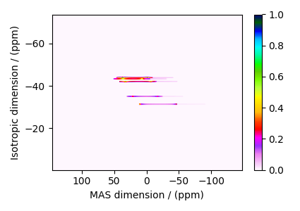
The plot of the simulation.

dataset = sim.methods[0].simulation

plt.figure(figsize=(4.25, 3.0))
ax = plt.subplot(projection="csdm")
cb = ax.imshow(dataset.real / dataset.real.max(), aspect="auto", cmap="gist_ncar_r")
plt.colorbar(cb)
ax.invert_xaxis()
ax.invert_yaxis()
plt.tight_layout()
plt.show()

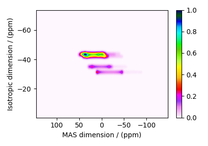
Add post-simulation signal processing.

processor = sp.SignalProcessor(
    operations=[
        # Gaussian convolution along both dimensions.
        sp.IFFT(dim_index=(0, 1)),
        sp.apodization.Gaussian(FWHM="0.3 kHz", dim_index=0),
        sp.apodization.Gaussian(FWHM="0.15 kHz", dim_index=1),
        sp.FFT(dim_index=(0, 1)),
    ]
)
processed_dataset = processor.apply_operations(dataset=dataset)
processed_dataset /= processed_dataset.max()

The plot of the simulation after signal processing.

plt.figure(figsize=(4.25, 3.0))
ax = plt.subplot(projection="csdm")
cb = ax.imshow(processed_dataset.real, cmap="gist_ncar_r", aspect="auto")
plt.colorbar(cb)
ax.invert_xaxis()
ax.invert_yaxis()
plt.tight_layout()
plt.show()

Total running time of the script: ( 0 minutes 0.846 seconds)

Gallery generated by Sphinx-Gallery