Coesite, ¹⁷O (I=5/2) DAS¶

¹⁷O (I=5/2) Dynamic-angle spinning (DAS) simulation.

The following is a Dynamic Angle Spinning (DAS) simulation of Coesite. Coesite has five crystallographic \(^{17}\text{O}\) sites. In the following, we use the \(^{17}\text{O}\) EFG tensor information from Grandinetti et al. [1]

import matplotlib.pyplot as plt
import numpy as np

from mrsimulator import Simulator
from mrsimulator import signal_processor as sp
from mrsimulator.method import Method, SpectralDimension, SpectralEvent

Create the Simulator object and load the spin systems database or url address.

sim = Simulator()

# load the spin systems from url.
filename = "https://ssnmr.org/sites/default/files/mrsimulator/coesite_0.mrsys"
sim.load_spin_systems(filename)

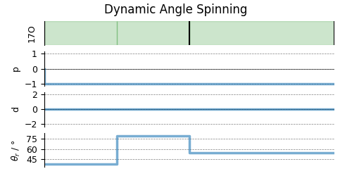
Use the generic method, Method, to simulate a 2D DAS spectrum by customizing the method parameters, as shown below.

das = Method(
    name="Dynamic Angle Spinning",
    channels=["17O"],
    magnetic_flux_density=11.74,  # in T
    rotor_frequency=np.inf,
    spectral_dimensions=[
        SpectralDimension(
            count=256,
            spectral_width=5e3,  # in Hz
            reference_offset=0,  # in Hz
            label="DAS isotropic dimension",
            events=[
                SpectralEvent(
                    fraction=0.5,
                    rotor_angle=37.38 * 3.14159 / 180,  # in rads
                    transition_queries=[{"ch1": {"P": [-1], "D": [0]}}],
                ),
                SpectralEvent(
                    fraction=0.5,
                    rotor_angle=79.19 * 3.14159 / 180,  # in rads
                    transition_queries=[{"ch1": {"P": [-1], "D": [0]}}],
                ),
            ],
        ),
        # The last spectral dimension block is the direct-dimension
        SpectralDimension(
            count=256,
            spectral_width=2e4,  # in Hz
            reference_offset=0,  # in Hz
            label="MAS dimension",
            events=[
                SpectralEvent(
                    rotor_angle=54.735 * 3.14159 / 180,  # in rads
                    transition_queries=[{"ch1": {"P": [-1], "D": [0]}}],
                )
            ],
        ),
    ],
)
sim.methods = [das]  # add the method

# A graphical representation of the method object.
plt.figure(figsize=(5, 2.5))
das.plot()
plt.show()

Run the simulation

sim.run()

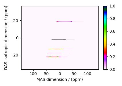
The plot of the simulation.

dataset = sim.methods[0].simulation

plt.figure(figsize=(4.25, 3.0))
ax = plt.subplot(projection="csdm")
cb = ax.imshow(dataset.real / dataset.real.max(), aspect="auto", cmap="gist_ncar_r")
plt.colorbar(cb)
ax.invert_xaxis()
ax.invert_yaxis()
plt.tight_layout()
plt.show()

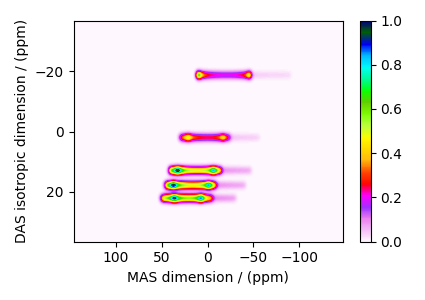
Add post-simulation signal processing.

processor = sp.SignalProcessor(
    operations=[
        # Gaussian convolution along both dimensions.
        sp.IFFT(dim_index=(0, 1)),
        sp.apodization.Gaussian(FWHM="0.3 kHz", dim_index=0),
        sp.apodization.Gaussian(FWHM="0.15 kHz", dim_index=1),
        sp.FFT(dim_index=(0, 1)),
    ]
)
processed_dataset = processor.apply_operations(dataset=dataset)
processed_dataset /= processed_dataset.max()

The plot of the simulation after signal processing.

plt.figure(figsize=(4.25, 3.0))
ax = plt.subplot(projection="csdm")
cb = ax.imshow(processed_dataset.real, cmap="gist_ncar_r", aspect="auto")
plt.colorbar(cb)
ax.invert_xaxis()
ax.invert_yaxis()
plt.tight_layout()
plt.show()

Total running time of the script: ( 0 minutes 1.024 seconds)

Gallery generated by Sphinx-Gallery