MCl₂.2D₂O, ²H (I=1) Shifting-d echo

²H (I=1) 2D NMR CSA-Quad 1st order correlation spectrum simulation.

The following is a static shifting-d echo NMR correlation simulation of \(\text{MCl}_2\cdot 2\text{D}_2\text{O}\) crystalline solid, where \(M \in [\text{Cu}, \text{Ni}, \text{Co}, \text{Fe}, \text{Mn}]\). The tensor parameters for the simulation and the corresponding spectrum are reported by Walder et al. [1].

import matplotlib.pyplot as plt

from mrsimulator import Simulator, SpinSystem, Site
from mrsimulator import signal_processor as sp
from mrsimulator.spin_system.tensors import SymmetricTensor
from mrsimulator.method import Method, SpectralDimension, SpectralEvent, MixingEvent

Generate the site and spin system objects.

site_Ni = Site(
    isotope="2H",
    isotropic_chemical_shift=-97,  # in ppm
    shielding_symmetric=SymmetricTensor(
        zeta=-551,  # in ppm
        eta=0.12,
        alpha=62 * 3.14159 / 180,  # in rads
        beta=114 * 3.14159 / 180,  # in rads
        gamma=171 * 3.14159 / 180,  # in rads
    ),
    quadrupolar=SymmetricTensor(Cq=77.2e3, eta=0.9),  # Cq in Hz
)

site_Cu = Site(
    isotope="2H",
    isotropic_chemical_shift=51,  # in ppm
    shielding_symmetric=SymmetricTensor(
        zeta=146,  # in ppm
        eta=0.84,
        alpha=95 * 3.14159 / 180,  # in rads
        beta=90 * 3.14159 / 180,  # in rads
        gamma=0 * 3.14159 / 180,  # in rads
    ),
    quadrupolar=SymmetricTensor(Cq=118.2e3, eta=0.8),  # Cq in Hz
)

site_Co = Site(
    isotope="2H",
    isotropic_chemical_shift=215,  # in ppm
    shielding_symmetric=SymmetricTensor(
        zeta=-1310,  # in ppm
        eta=0.23,
        alpha=180 * 3.14159 / 180,  # in rads
        beta=90 * 3.14159 / 180,  # in rads
        gamma=90 * 3.14159 / 180,  # in rads
    ),
    quadrupolar=SymmetricTensor(Cq=114.6e3, eta=0.95),  # Cq in Hz
)

site_Fe = Site(
    isotope="2H",
    isotropic_chemical_shift=101,  # in ppm
    shielding_symmetric=SymmetricTensor(
        zeta=-1187,  # in ppm
        eta=0.4,
        alpha=122 * 3.14159 / 180,  # in rads
        beta=90 * 3.14159 / 180,  # in rads
        gamma=90 * 3.14159 / 180,  # in rads
    ),
    quadrupolar=SymmetricTensor(Cq=114.2e3, eta=0.98),  # Cq in Hz
)

site_Mn = Site(
    isotope="2H",
    isotropic_chemical_shift=145,  # in ppm
    shielding_symmetric=SymmetricTensor(
        zeta=-1236,  # in ppm
        eta=0.23,
        alpha=136 * 3.14159 / 180,  # in rads
        beta=90 * 3.14159 / 180,  # in rads
        gamma=90 * 3.14159 / 180,  # in rads
    ),
    quadrupolar=SymmetricTensor(Cq=1.114e5, eta=1.0),  # Cq in Hz
)

spin_systems = [
    SpinSystem(sites=[s], name=f"{n}Cl$_2$.2D$_2$O")
    for s, n in zip(
        [site_Ni, site_Cu, site_Co, site_Fe, site_Mn], ["Ni", "Cu", "Co", "Fe", "Mn"]
    )
]

Use the generic method, Method, to generate a 2D shifting-d echo method. The reported shifting-d 2D sequence is a correlation of the shielding frequencies to the first-order quadrupolar frequencies. Here, we create a correlation method using the freq_contrib attribute, which acts as a switch for including the frequency contributions from interaction during the event.

In the following method, we assign the ["Quad1_2"] and ["Shielding1_0", "Shielding1_2"] as the value to the freq_contrib key. The Quad1_2 is an enumeration for selecting the first-order second-rank quadrupolar frequency contributions. Shielding1_0 and Shielding1_2 are enumerations for the first-order shielding with zeroth and second-rank tensor contributions, respectively. See FrequencyEnum for details.

Like the previous example, we stipulate no mixing between the two spectral events using a MixingEvent with NoMixing as the query. Since all spin systems in this example have a single site, defining no mixing between the two spectral events is superfluous, but we include it so this method may be used with multi-site spin systems.

shifting_d = Method(
    name="Shifting-d",
    channels=["2H"],
    magnetic_flux_density=9.395,  # in T
    rotor_frequency=0,  # in Hz
    spectral_dimensions=[
        SpectralDimension(
            count=512,
            spectral_width=2.5e5,  # in Hz
            label="Quadrupolar frequency",
            events=[
                SpectralEvent(
                    transition_queries=[{"ch1": {"P": [-1]}}],
                    freq_contrib=["Quad1_2"],
                ),
                MixingEvent(query="NoMixing"),
            ],
        ),
        SpectralDimension(
            count=256,
            spectral_width=2e5,  # in Hz
            reference_offset=2e4,  # in Hz
            label="Paramagnetic shift",
            events=[
                SpectralEvent(
                    transition_queries=[{"ch1": {"P": [-1]}}],
                    freq_contrib=["Shielding1_0", "Shielding1_2"],
                )
            ],
        ),
    ],
)

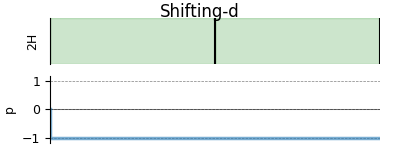
# A graphical representation of the method object.
plt.figure(figsize=(4, 1.5))
shifting_d.plot()
plt.show()

Create the Simulator object, add the method and spin system objects, and run the simulation.

sim = Simulator(spin_systems=spin_systems, methods=[shifting_d])
# Configure the simulator object. For non-coincidental tensors, set the value of the
# `integration_volume` attribute to `hemisphere`.
sim.config.integration_volume = "hemisphere"
sim.config.decompose_spectrum = "spin_system"  # simulate spectra per spin system
sim.run()

Add post-simulation signal processing.

dataset = sim.methods[0].simulation
processor = sp.SignalProcessor(
    operations=[
        # Gaussian convolution along both dimensions.
        sp.IFFT(dim_index=(0, 1)),
        sp.apodization.Gaussian(FWHM="9 kHz", dim_index=0),  # along dimension 0
        sp.apodization.Gaussian(FWHM="9 kHz", dim_index=1),  # along dimension 1
        sp.FFT(dim_index=(0, 1)),
    ]
)
processed_dataset = processor.apply_operations(dataset=dataset)

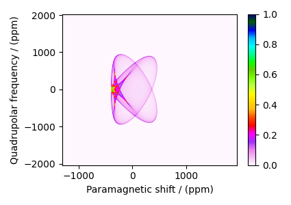
The plot of the simulation. Because we configured the simulator object to simulate spectrum per spin system, the following dataset is a CSDM object containing five simulations (dependent variables). Let’s visualize the first dataset corresponding to \(\text{NiCl}_2\cdot 2 \text{D}_2\text{O}\).

dataset_Ni = dataset.split()[0].real

plt.figure(figsize=(4.25, 3.0))
ax = plt.subplot(projection="csdm")
cb = ax.imshow(dataset_Ni / dataset_Ni.max(), aspect="auto", cmap="gist_ncar_r")
plt.title(None)
plt.colorbar(cb)
plt.tight_layout()
plt.show()

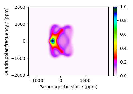
The plot of the simulation after signal processing.

proc_dataset_Ni = processed_dataset.split()[0].real

plt.figure(figsize=(4.25, 3.0))
ax = plt.subplot(projection="csdm")
cb = ax.imshow(
    proc_dataset_Ni / proc_dataset_Ni.max(), cmap="gist_ncar_r", aspect="auto"
)
plt.title(None)
plt.colorbar(cb)
plt.tight_layout()
plt.show()

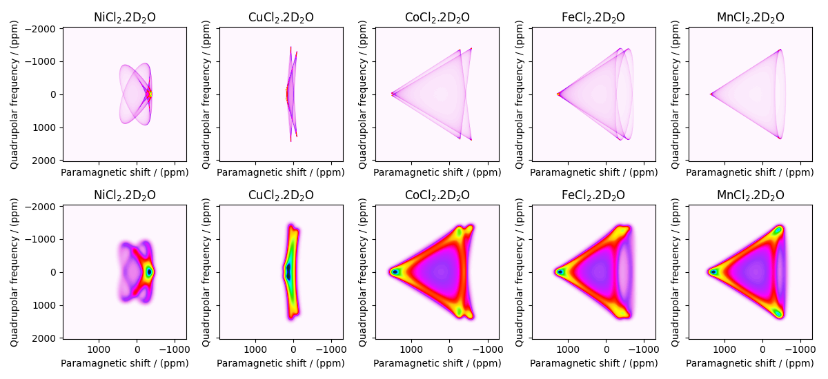
Let’s plot all the simulated datasets.

fig, ax = plt.subplots(
    2, 5, sharex=True, sharey=True, figsize=(12, 5.5), subplot_kw={"projection": "csdm"}
)
for i, dataset_obj in enumerate([dataset, processed_dataset]):
    for j, datum in enumerate(dataset_obj.split()):
        ax[i, j].imshow((datum / datum.max()).real, aspect="auto", cmap="gist_ncar_r")
        ax[i, j].invert_xaxis()
        ax[i, j].invert_yaxis()

plt.tight_layout()
plt.show()

[1]

Walder B.J, Patterson A.M., Baltisberger J.H, and Grandinetti P.J Hydrogen motional disorder in crystalline iron group chloride di-hydrates spectroscopy, J. Chem. Phys. (2018) 149, 084503. DOI: 10.1063/1.5037151