Note
Go to the end to download the full example code.
1D PASS/MAT sideband order cross-section
This example illustrates the use of mrsimulator and LMFIT modules in fitting the sideband intensity profile across the isotropic chemical shift cross-section from a PASS/MAT dataset.
import csdmpy as cp
import matplotlib.pyplot as plt
from lmfit import Minimizer

from mrsimulator import Simulator, SpinSystem, Site
from mrsimulator.method.lib import BlochDecaySpectrum
from mrsimulator import signal_processor as sp
from mrsimulator.utils import spectral_fitting as sf
from mrsimulator.utils import get_spectral_dimensions
from mrsimulator.spin_system.tensors import SymmetricTensor
Import the dataset
name = "https://ssnmr.org/sites/default/files/mrsimulator/LHistidine_cross_section.csdf"
pass_cross_section = cp.load(name)
# standard deviation of noise from the dataset
sigma = 4.640351
# For the spectral fitting, we only focus on the real part of the complex dataset.
pass_cross_section = pass_cross_section.real
# Convert the coordinates along each dimension from Hz to ppm.
_ = [item.to("ppm", "nmr_frequency_ratio") for item in pass_cross_section.dimensions]
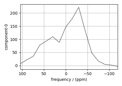
# The plot of the dataset.
plt.figure(figsize=(4.25, 3.0))
ax = plt.subplot(projection="csdm")
ax.plot(pass_cross_section, "k", alpha=0.5)
ax.invert_xaxis()
plt.grid()
plt.tight_layout()
plt.show()
Create a fitting model
Guess model
Create a guess list of spin systems. For fitting the sideband profile at an isotropic chemical shift cross-section from PASS/MAT datasets, set the isotropic_chemical_shift parameter of the site object as zero.
site = Site(
    isotope="13C",
    isotropic_chemical_shift=0,  #
    shielding_symmetric=SymmetricTensor(zeta=-70, eta=0.8),
)
spin_systems = [SpinSystem(sites=[site])]
Method
For the sideband-only cross-section, use the BlochDecaySpectrum method.
# Get the dimension information from the experiment.
spectral_dims = get_spectral_dimensions(pass_cross_section)

PASS = BlochDecaySpectrum(
    channels=["13C"],
    magnetic_flux_density=9.395,  # in T
    rotor_frequency=1500,  # in Hz
    spectral_dimensions=spectral_dims,
    experiment=pass_cross_section,  # also add the measurement to the method.
)
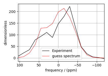
Guess Spectrum
# Simulation
# ----------
sim = Simulator(spin_systems=spin_systems, methods=[PASS])
sim.run()

# Post Simulation Processing
# --------------------------
processor = sp.SignalProcessor(operations=[sp.Scale(factor=20000)])
processed_dataset = processor.apply_operations(dataset=sim.methods[0].simulation).real

# Plot of the guess Spectrum
# --------------------------
plt.figure(figsize=(4.25, 3.0))
ax = plt.subplot(projection="csdm")
ax.plot(pass_cross_section, color="k", linewidth=1, label="Experiment")
ax.plot(processed_dataset, color="r", alpha=0.75, linewidth=1, label="guess spectrum")
plt.grid()
ax.invert_xaxis()
plt.legend()
plt.tight_layout()
plt.show()
Least-squares minimization with LMFIT
First, create the fitting parameters.
Use the make_LMFIT_params() for a quick
setup.
params = sf.make_LMFIT_params(sim, processor)

# Fix the value of the isotropic chemical shift to zero for pure anisotropic sideband
# amplitude simulation.
params["sys_0_site_0_isotropic_chemical_shift"].vary = False
print(params.pretty_print(columns=["value", "min", "max", "vary", "expr"]))
Name                                      Value      Min      Max     Vary     Expr
SP_0_operation_0_Scale_factor             2e+04     -inf      inf     True     None
sys_0_abundance                             100        0      100    False      100
sys_0_site_0_isotropic_chemical_shift         0     -inf      inf    False     None
sys_0_site_0_shielding_symmetric_eta        0.8        0        1     True     None
sys_0_site_0_shielding_symmetric_zeta       -70     -inf      inf     True     None
None
Run the minimization using LMFIT
opt = sim.optimize()
minner = Minimizer(
    sf.LMFIT_min_function,
    params,
    fcn_args=(sim, processor, sigma),
    fcn_kws={"opt": opt},
)
result = minner.minimize()
result
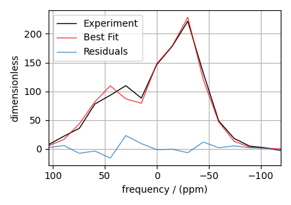
The best fit solution
best_fit = sf.bestfit(sim, processor)[0].real
residuals = sf.residuals(sim, processor)[0].real

# Plot the spectrum
plt.figure(figsize=(4.25, 3.0))
ax = plt.subplot(projection="csdm")
ax.plot(pass_cross_section, color="k", linewidth=1, label="Experiment")
ax.plot(best_fit, "r", alpha=0.75, linewidth=1, label="Best Fit")
ax.plot(residuals, alpha=0.75, linewidth=1, label="Residuals")
ax.invert_xaxis()
plt.grid()
plt.legend()
plt.tight_layout()
plt.show()
Total running time of the script: (0 minutes 1.431 seconds)