Note
Go to the end to download the full example code.
Polynomial Offset
In this example, we will use the
Polynomial class to
offset the baseline of a dataset by a polynomial function.
Below we import the necessary modules
import csdmpy as cp
import numpy as np
from mrsimulator import signal_processor as sp
First we create processor, an instance of the
SignalProcessor class. The required
attribute of the SignalProcessor class, operations, is a list of operations to which
we add a Polynomial object.
The required argument for the polynomial offset is polynomial_dictionary which is a Python dict defining the polynomial coefficients. An arbitrary number of coefficients may be passed.
processor = sp.SignalProcessor(
    operations=[
        sp.baseline.Polynomial(polynomial_dictionary={"c0": 0.2, "c2": 0.00001})
    ]
)
Here the applied offset will be the following function
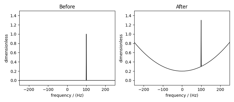
Next we create a CSDM object with a test dataset which our signal processor will operate on. Here, the dataset spans 500 Hz with a delta function centered at 100 Hz.
test_data = np.zeros(500)
test_data[350] = 1
csdm_object = cp.CSDM(
    dependent_variables=[cp.as_dependent_variable(test_data)],
    dimensions=[cp.LinearDimension(count=500, increment="1 Hz", complex_fft=True)],
)
Now to apply the processor to the CSDM object, use the
apply_operations() method as
follows
processed_dataset = processor.apply_operations(dataset=csdm_object.copy()).real
To see the results of the exponential apodization, we create a simple plot using the
matplotlib library.
import matplotlib.pyplot as plt

fig, ax = plt.subplots(1, 2, figsize=(8, 3.5), subplot_kw={"projection": "csdm"})
ax[0].plot(csdm_object, color="black", linewidth=1)
ax[0].set(ylim=(-0.1, 1.5))
ax[0].set_title("Before")
ax[1].plot(processed_dataset.real, color="black", linewidth=1)
ax[1].set(ylim=(-0.1, 1.5))
ax[1].set_title("After")
plt.tight_layout()
plt.show()
Total running time of the script: (0 minutes 0.413 seconds)