Top-Hat Apodization

In this example, we will use the TopHat class to apply a point-wise top hat apodization on the Fourier transform of an example dataset. The function is defined as follows

(48)\[\begin{split}f(x) = \begin{cases} 1, \tt{rising\_edge} \leq x \leq \tt{falling\_edge} \\ 0, \text{otherwise} \end{cases}\end{split}\]

where rising_edge is the start of the window and falling_edge is the end of the window.

When falling_edge is undefined, all points after rising_edge will be 1. Similarly, when rising_edge is undefined, all points before falling_edge are 1.

Below we import the necessary modules

import csdmpy as cp
import matplotlib.pyplot as plt
import numpy as np
from mrsimulator import signal_processor as sp

First we create processor, and instance of the SignalProcessor class. The required attribute of the SignalProcessor class, operations, is a list of operations to which we add a TopHat object sandwiched between two Fourier transformations. Here the window is between 1 and 9 seconds.

processor = sp.SignalProcessor(
    operations=[
        sp.IFFT(),
        sp.apodization.TopHat(rising_edge="1 s", falling_edge="9 s"),
        sp.FFT(),
    ]
)

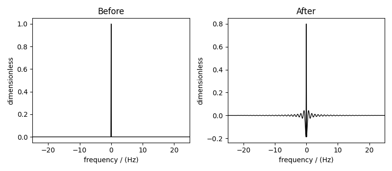
Next we create a CSDM object with a test dataset which our signal processor will operate on. Here, the dataset is a delta function centered at 0 Hz with a some applied Gaussian line broadening.

test_data = np.zeros(500)
test_data[250] = 1
csdm_object = cp.CSDM(
    dependent_variables=[cp.as_dependent_variable(test_data)],
    dimensions=[cp.LinearDimension(count=500, increment="0.1 Hz", complex_fft=True)],
)

To apply the previously defined signal processor, we use the apply_operations() method as as follows

processed_dataset = processor.apply_operations(dataset=csdm_object).real

To see the results of the top hat apodization, we create a simple plot using the matplotlib library.

fig, ax = plt.subplots(1, 2, figsize=(8, 3.5), subplot_kw={"projection": "csdm"})
ax[0].plot(csdm_object, color="black", linewidth=1)
ax[0].set_title("Before")
ax[1].plot(processed_dataset.real, color="black", linewidth=1)
ax[1].set_title("After")
plt.tight_layout()
plt.show()

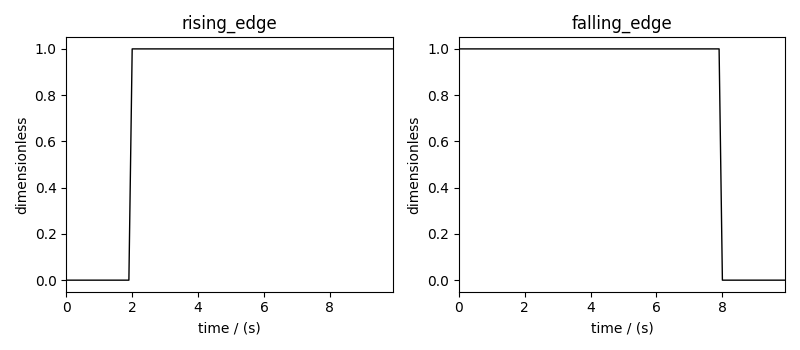
Below are plots showing how the apodization functions when only rising_edge or falling_edge are defined.

rising_edge_processor = sp.SignalProcessor(
    operations=[sp.apodization.TopHat(rising_edge="2 s")]
)
falling_edge_processor = sp.SignalProcessor(
    operations=[sp.apodization.TopHat(falling_edge="8 s")]
)

constant_csdm = cp.CSDM(
    dependent_variables=[cp.as_dependent_variable(np.ones(100))],
    dimensions=[cp.LinearDimension(100, increment="0.1 s")],
)
rising_dataset = rising_edge_processor.apply_operations(
    dataset=constant_csdm.copy()
).real
falling_dataset = falling_edge_processor.apply_operations(
    dataset=constant_csdm.copy()
).real

fig, ax = plt.subplots(1, 2, figsize=(8, 3.5), subplot_kw={"projection": "csdm"})
ax[0].plot(rising_dataset, color="black", linewidth=1)
ax[0].set_title("rising_edge")
ax[1].plot(falling_dataset, color="black", linewidth=1)
ax[1].set_title("falling_edge")
plt.tight_layout()
plt.show()