Rb2SO4, 87Rb (I=3/2) SAS

87Rb (I=3/2) Switched-angle spinning (SAS) simulation.

The following is an example of switched-angle spinning (SAS) simulation of \(\text{Rb}_2\text{SO}_4\), which has two distinct rubidium sites. The NMR tensor parameters for these sites are taken from Shore et. al. 1.

import matplotlib as mpl
import matplotlib.pyplot as plt
import mrsimulator.signal_processing as sp
import mrsimulator.signal_processing.apodization as apo
from mrsimulator import Simulator, SpinSystem, Site
from mrsimulator.methods import Method2D

# global plot configuration
font = {"size": 9}
mpl.rc("font", **font)
mpl.rcParams["figure.figsize"] = [4.25, 3.0]

Generate the site and spin system objects.

sites = [
    Site(
        isotope="87Rb",
        isotropic_chemical_shift=16,  # in ppm
        quadrupolar={"Cq": 5.3e6, "eta": 0.1},  # Cq in Hz
    ),
    Site(
        isotope="87Rb",
        isotropic_chemical_shift=40,  # in ppm
        quadrupolar={"Cq": 2.6e6, "eta": 1.0},  # Cq in Hz
    ),
]
spin_systems = [SpinSystem(sites=[s]) for s in sites]

Use the generic 2D method, Method2D, to simulate a SAS spectrum by customizing the method parameters, as shown below. Note, the Method2D method simulates an infinite spinning speed spectrum.

sas = Method2D(
    channels=["87Rb"],
    magnetic_flux_density=9.4,  # in T
    spectral_dimensions=[
        {
            "count": 256,
            "spectral_width": 3.5e4,  # in Hz
            "reference_offset": 1e3,  # in Hz
            "label": "90 dimension",
            "events": [{"rotor_angle": 90 * 3.14159 / 180}],  # in radians
        },
        {
            "count": 256,
            "spectral_width": 22e3,  # in Hz
            "reference_offset": -4e3,  # in Hz
            "label": "MAS dimension",
            "events": [{"rotor_angle": 54.74 * 3.14159 / 180}],  # in radians
        },
    ],
)

Create the Simulator object, add the method and spin system objects, and run the simulation.

sim = Simulator()
sim.spin_systems = spin_systems  # add the spin systems
sim.methods = [sas]  # add the method.
sim.run()

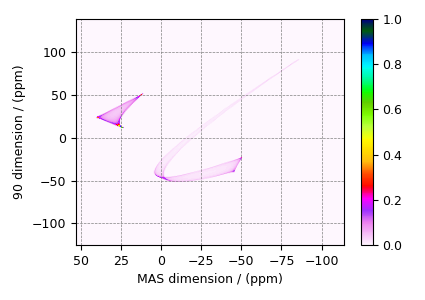
The plot of the simulation.

data = sim.methods[0].simulation
ax = plt.subplot(projection="csdm")
cb = ax.imshow(data / data.max(), aspect="auto", cmap="gist_ncar_r")
plt.colorbar(cb)
ax.invert_xaxis()
plt.tight_layout()
plt.show()

Add post-simulation signal processing.

processor = sp.SignalProcessor(
    operations=[
        # Gaussian convolution along both dimensions.
        sp.IFFT(dim_index=(0, 1)),
        apo.Gaussian(FWHM="0.4 kHz", dim_index=0),
        apo.Gaussian(FWHM="0.4 kHz", dim_index=1),
        sp.FFT(dim_index=(0, 1)),
    ]
)
processed_data = processor.apply_operations(data=data)
processed_data /= processed_data.max()

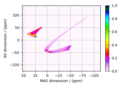
The plot of the simulation after signal processing.

ax = plt.subplot(projection="csdm")
cb = ax.imshow(processed_data.real, cmap="gist_ncar_r", aspect="auto")
plt.colorbar(cb)
ax.invert_xaxis()
plt.tight_layout()
plt.show()

1

Shore, J.S., Wang, S.H., Taylor, R.E., Bell, A.T., Pines, A. Determination of quadrupolar and chemical shielding tensors using solid-state two-dimensional NMR spectroscopy, J. Chem. Phys. (1996) 105 21, 9412. DOI: 10.1063/1.472776