Coesite, 17O (I=5/2) DAS

17O (I=5/2) Dynamic-angle spinning (DAS) simulation.

The following is a dynamic angle spinning (DAS) simulation of Coesite. Coesite has five crystallographic \(^{17}\text{O}\) sites. In the following, we use the \(^{17}\text{O}\) EFG tensor information from Grandinetti et. al. 1

import matplotlib as mpl
import matplotlib.pyplot as plt
import mrsimulator.signal_processing as sp
import mrsimulator.signal_processing.apodization as apo
from mrsimulator import Simulator
from mrsimulator.methods import Method2D

# global plot configuration
font = {"size": 9}
mpl.rc("font", **font)
mpl.rcParams["figure.figsize"] = [4.25, 3.0]

Create the Simulator object and load the spin systems database or url address.

sim = Simulator()

# load the spin systems from url.
filename = "https://sandbox.zenodo.org/record/687656/files/coesite.mrsys"
sim.load_spin_systems(filename)

Use the generic 2D method, Method2D, to simulate a DAS spectrum by customizing the method parameters, as shown below. Note, the Method2D method simulates an infinite spinning speed spectrum.

das = Method2D(
    channels=["17O"],
    magnetic_flux_density=11.7,  # in T
    spectral_dimensions=[
        {
            "count": 256,
            "spectral_width": 5e3,  # in Hz
            "reference_offset": 0,  # in Hz
            "label": "DAS isotropic dimension",
            "events": [
                {"fraction": 0.5, "rotor_angle": 37.38 * 3.14159 / 180},
                {"fraction": 0.5, "rotor_angle": 79.19 * 3.14159 / 180},
            ],
        },
        # The last spectral dimension block is the direct-dimension
        {
            "count": 256,
            "spectral_width": 2e4,  # in Hz
            "reference_offset": 0,  # in Hz
            "label": "MAS dimension",
            "events": [{"rotor_angle": 54.735 * 3.14159 / 180}],
        },
    ],
)
sim.methods = [das]  # add the method.

Run the simulation

sim.run()

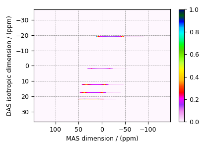
The plot of the simulation.

data = sim.methods[0].simulation
ax = plt.subplot(projection="csdm")
cb = ax.imshow(data / data.max(), aspect="auto", cmap="gist_ncar_r")
plt.colorbar(cb)
ax.invert_xaxis()
ax.invert_yaxis()
plt.tight_layout()
plt.show()

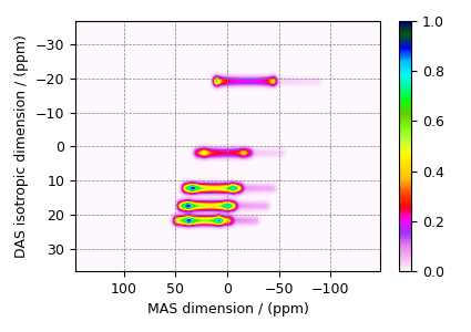
Add post-simulation signal processing.

processor = sp.SignalProcessor(
    operations=[
        # Gaussian convolution along both dimensions.
        sp.IFFT(dim_index=(0, 1)),
        apo.Gaussian(FWHM="0.3 kHz", dim_index=0),
        apo.Gaussian(FWHM="0.15 kHz", dim_index=1),
        sp.FFT(dim_index=(0, 1)),
    ]
)
processed_data = processor.apply_operations(data=data)
processed_data /= processed_data.max()

The plot of the simulation after signal processing.

ax = plt.subplot(projection="csdm")
cb = ax.imshow(processed_data.real, cmap="gist_ncar_r", aspect="auto")
plt.colorbar(cb)
ax.invert_xaxis()
ax.invert_yaxis()
plt.tight_layout()
plt.show()

1

Grandinetti, P. J., Baltisberger, J. H., Farnan, I., Stebbins, J. F., Werner, U. and Pines, A. Solid-State \(^{17}\text{O}\) Magic-Angle and Dynamic-Angle Spinning NMR Study of the \(\text{SiO}_2\) Polymorph Coesite, J. Phys. Chem. 1995, 99, 32, 12341-12348. DOI: 10.1021/j100032a045