Rb2CrO4, 87Rb (I=3/2) COASTER

87Rb (I=3/2) Correlation of anisotropies separated through echo refocusing (COASTER) simulation.

The following is a correlation of anisotropies separated through echo refocusing (COASTER) simulation of \(\text{Rb}_2\text{CrO}_4\). The Rb site with the smaller quadrupolar interaction is selectively observed and reported by Ash et. al. 1. The following is the simulation based on the published tensor parameters.

import matplotlib as mpl
import matplotlib.pyplot as plt
import mrsimulator.signal_processing as sp
import mrsimulator.signal_processing.apodization as apo
from mrsimulator import Simulator, SpinSystem, Site
from mrsimulator.methods import Method2D

# global plot configuration
font = {"size": 9}
mpl.rc("font", **font)
mpl.rcParams["figure.figsize"] = [4.25, 3.0]

Generate the site and spin system objects.

site = Site(
    isotope="87Rb",
    isotropic_chemical_shift=-9,  # in ppm
    shielding_symmetric={"zeta": 110, "eta": 0},
    quadrupolar={
        "Cq": 3.5e6,  # in Hz
        "eta": 0.36,
        "alpha": 0,  # in rads
        "beta": 70 * 3.14159 / 180,  # in rads
        "gamma": 0,  # in rads
    },
)
spin_system = SpinSystem(sites=[site])

Use the generic 2D method, Method2D, to simulate a COASTER spectrum by customizing the method parameters, as shown below. Note, the Method2D method simulates an infinite spinning speed spectrum.

coaster = Method2D(
    channels=["87Rb"],
    magnetic_flux_density=9.4,  # in T
    rotor_angle=70.12 * 3.14159 / 180,  # in rads
    spectral_dimensions=[
        {
            "count": 256,
            "spectral_width": 4e4,  # in Hz
            "reference_offset": -8e3,  # in Hz
            "label": "3Q dimension",
            "events": [{"transition_query": {"P": [3], "D": [0]}}],
        },
        # The last spectral dimension block is the direct-dimension
        {
            "count": 256,
            "spectral_width": 2e4,  # in Hz
            "reference_offset": -3e3,  # in Hz
            "label": "70.12 dimension",
            "events": [{"transition_query": {"P": [-1], "D": [0]}}],
        },
    ],
)

Create the Simulator object, add the method and spin system objects, and run the simulation.

sim = Simulator()
sim.spin_systems = [spin_system]  # add the spin systems
sim.methods = [coaster]  # add the method.

# configure the simulator object. For non-coincidental tensors, set the value of the
# `integration_volume` attribute to `hemisphere`.
sim.config.integration_volume = "hemisphere"
sim.run()

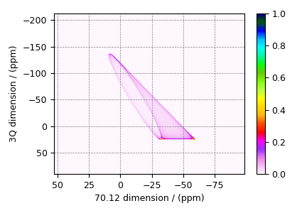
The plot of the simulation.

data = sim.methods[0].simulation
ax = plt.subplot(projection="csdm")
cb = ax.imshow(data / data.max(), aspect="auto", cmap="gist_ncar_r")
plt.colorbar(cb)
ax.invert_xaxis()
ax.invert_yaxis()
plt.tight_layout()
plt.show()

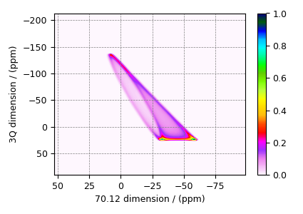
Add post-simulation signal processing.

processor = sp.SignalProcessor(
    operations=[
        # Gaussian convolution along both dimensions.
        sp.IFFT(dim_index=(0, 1)),
        apo.Gaussian(FWHM="0.3 kHz", dim_index=0),
        apo.Gaussian(FWHM="0.3 kHz", dim_index=1),
        sp.FFT(dim_index=(0, 1)),
    ]
)
processed_data = processor.apply_operations(data=data)
processed_data /= processed_data.max()

The plot of the simulation after signal processing.

ax = plt.subplot(projection="csdm")
cb = ax.imshow(processed_data.real, cmap="gist_ncar_r", aspect="auto")
plt.colorbar(cb)
ax.invert_xaxis()
ax.invert_yaxis()
plt.tight_layout()
plt.show()

1

Jason T. Ash, Nicole M. Trease, and Philip J. Grandinetti. Separating Chemical Shift and Quadrupolar Anisotropies via Multiple-Quantum NMR Spectroscopy, J. Am. Chem. Soc. (2008) 130, 10858-10859. DOI: 10.1021/ja802865x