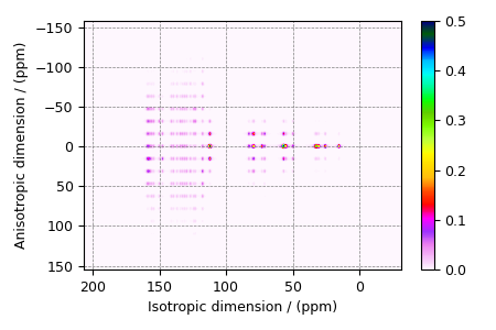
Itraconazole, 13C (I=1/2) PASS

13C (I=1/2) 2D Phase-adjusted spinning sideband (PASS) simulation.

The following is a simulation of a 2D PASS spectrum of itraconazole, a triazole containing drug prescribed for the prevention and treatment of fungal infection. The 2D PASS spectrum is a correlation of finite speed MAS to an infinite speed MAS spectrum. The parameters for the simulation are obtained from Dey et. al. 1.

import matplotlib as mpl
import matplotlib.pyplot as plt
import mrsimulator.signal_processing as sp
import mrsimulator.signal_processing.apodization as apo
from mrsimulator import Simulator
from mrsimulator.methods import SSB2D

# global plot configuration
font = {"size": 9}
mpl.rc("font", **font)
mpl.rcParams["figure.figsize"] = [4.5, 3.0]

There are 41 \(^{13}\text{C}\) single-site spin systems partially describing the NMR parameters of itraconazole. We will import the directly import the spin systems to the Simulator object using the load_spin_systems method.

sim = Simulator()

filename = "https://sandbox.zenodo.org/record/687656/files/itraconazole_13C.mrsys"
sim.load_spin_systems(filename)

Use the SSB2D method to simulate a PASS, MAT, QPASS, QMAT, or any equivalent sideband separation spectrum. Here, we use the method to generate a PASS spectrum.

PASS = SSB2D(
    channels=["13C"],
    magnetic_flux_density=11.74,
    rotor_frequency=2000,
    spectral_dimensions=[
        {
            "count": 20 * 4,
            "spectral_width": 2000 * 20,  # value in Hz
            "label": "Anisotropic dimension",
        },
        {
            "count": 1024,
            "spectral_width": 3e4,  # value in Hz
            "reference_offset": 1.1e4,  # value in Hz
            "label": "Isotropic dimension",
        },
    ],
)
sim.methods = [PASS]  # add the method.

# For 2D spinning sideband simulation, set the number of spinning sidebands in the
# Simulator.config object to `spectral_width/rotor_frequency` along the sideband
# dimension.
sim.config.number_of_sidebands = 20

# run the simulation.
sim.run()

Apply post-simulation processing. Here, we apply a Lorentzian line broadening to the isotropic dimension.

data = sim.methods[0].simulation
processor = sp.SignalProcessor(
    operations=[
        sp.IFFT(dim_index=0),
        apo.Exponential(FWHM="100 Hz", dim_index=0),
        sp.FFT(dim_index=0),
    ]
)
processed_data = processor.apply_operations(data=data).real
processed_data /= processed_data.max()

The plot of the simulation.

ax = plt.subplot(projection="csdm")
cb = ax.imshow(processed_data, aspect="auto", cmap="gist_ncar_r", vmax=0.5)
plt.colorbar(cb)
ax.invert_xaxis()
ax.invert_yaxis()
plt.tight_layout()
plt.show()

1

Dey, K .K, Gayen, S., Ghosh, M., Investigation of the Detailed Internal Structure and Dynamics of Itraconazole by Solid-State NMR Measurements, ACS Omega (2019) 4, 21627. DOI:10.1021/acsomega.9b03558