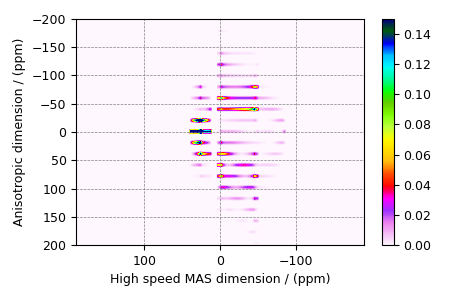
Rb2SO4, 87Rb (I=3/2) QMAT

87Rb (I=3/2) Quadrupolar Magic-angle turning (QMAT) simulation.

The following is a simulation of the QMAT spectrum of \(\text{Rb}_2\text{SiO}_4\). The 2D QMAT spectrum is a correlation of finite speed MAS to an infinite speed MAS spectrum. The parameters for the simulation are obtained from Walder et. al. 1.

import matplotlib as mpl
import matplotlib.pyplot as plt
from mrsimulator import Simulator, SpinSystem, Site
from mrsimulator.methods import SSB2D

# global plot configuration
font = {"size": 9}
mpl.rc("font", **font)
mpl.rcParams["figure.figsize"] = [4.5, 3.0]

Generate the site and spin system objects.

sites = [
    Site(
        isotope="87Rb",
        isotropic_chemical_shift=16,  # in ppm
        quadrupolar={"Cq": 5.3e6, "eta": 0.1},  # Cq in Hz
    ),
    Site(
        isotope="87Rb",
        isotropic_chemical_shift=40,  # in ppm
        quadrupolar={"Cq": 2.6e6, "eta": 1.0},  # Cq in Hz
    ),
]
spin_systems = [SpinSystem(sites=[s]) for s in sites]

Use the SSB2D method to simulate a PASS, MAT, QPASS, QMAT, or any equivalent sideband separation spectrum. Here, we use the method to generate a QMAT spectrum. The QMAT method is created from the SSB2D method in the same as a PASS or MAT method. The difference is that the observed channel is a half-integer quadrupolar spin instead of a spin I=1/2.

qmat = SSB2D(
    channels=["87Rb"],
    magnetic_flux_density=9.4,
    rotor_frequency=2604,
    spectral_dimensions=[
        {
            "count": 32 * 4,
            "spectral_width": 2604 * 32,  # in Hz
            "label": "Anisotropic dimension",
        },
        {
            "count": 512,
            "spectral_width": 50000,  # in Hz
            "label": "High speed MAS dimension",
        },
    ],
)

Create the Simulator object, add the method and spin system objects, and run the simulation.

sim = Simulator()
sim.spin_systems = spin_systems  # add the spin systems
sim.methods = [qmat]  # add the method.

# For 2D spinning sideband simulation, set the number of spinning sidebands in the
# Simulator.config object to `spectral_width/rotor_frequency` along the sideband
# dimension.
sim.config.number_of_sidebands = 32
sim.run()

The plot of the simulation.

data = sim.methods[0].simulation
ax = plt.subplot(projection="csdm")
cb = ax.imshow(data / data.max(), aspect="auto", cmap="gist_ncar_r", vmax=0.15)
plt.colorbar(cb)
ax.invert_xaxis()
ax.set_ylim(200, -200)
plt.tight_layout()
plt.show()

1

Walder, B. J., Dey, K .K, Kaseman, D. C., Baltisberger, J. H., and Philip J. Grandinetti. Sideband separation experiments in NMR with phase incremented echo train acquisition, J. Chem. Phys. (2013) 138, 174203. DOI:10.1063/1.4803142