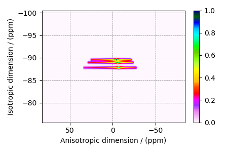
Wollastonite, 29Si (I=1/2), MAF

29Si (I=1/2) magic angle flipping.

Wollastonite is a high-temperature calcium-silicate, \(\beta−\text{Ca}_3\text{Si}_3\text{O}_9\), with three distinct \(^{29}\text{Si}\) sites. The \(^{29}\text{Si}\) tensor parameters were obtained from Hansen et. al. 1

import matplotlib as mpl
import matplotlib.pyplot as plt
import mrsimulator.signal_processing as sp
import mrsimulator.signal_processing.apodization as apo
from mrsimulator import Simulator, SpinSystem, Site
from mrsimulator.methods import Method2D

# global plot configuration
mpl.rcParams["figure.figsize"] = [4.5, 3.0]

Create the sites and spin systems

sites = [
    Site(
        isotope="29Si",
        isotropic_chemical_shift=-89.0,  # in ppm
        shielding_symmetric={"zeta": 59.8, "eta": 0.62},  # zeta in ppm
    ),
    Site(
        isotope="29Si",
        isotropic_chemical_shift=-89.5,  # in ppm
        shielding_symmetric={"zeta": 52.1, "eta": 0.68},  # zeta in ppm
    ),
    Site(
        isotope="29Si",
        isotropic_chemical_shift=-87.8,  # in ppm
        shielding_symmetric={"zeta": 69.4, "eta": 0.60},  # zeta in ppm
    ),
]

spin_systems = [SpinSystem(sites=[s]) for s in sites]

Use the generic 2D method, Method2D, to simulate a MAF spectrum by customizing the method parameters, as shown below. Note, the Method2D method simulates an infinite spinning speed spectrum.

maf = Method2D(
    channels=["29Si"],
    magnetic_flux_density=14.1,  # in T
    spectral_dimensions=[
        {
            "count": 128,
            "spectral_width": 2e4,  # in Hz
            "label": "Anisotropic dimension",
            "events": [{"rotor_angle": 90 * 3.14159 / 180}],
        },
        {
            "count": 128,
            "spectral_width": 3e3,  # in Hz
            "reference_offset": -1.05e4,  # in Hz
            "label": "Isotropic dimension",
            "events": [{"rotor_angle": 54.735 * 3.14159 / 180}],
        },
    ],
    affine_matrix=[[1, -1], [0, 1]],
)

Create the Simulator object, add the method and spin system objects, and run the simulation.

sim = Simulator()
sim.spin_systems = spin_systems  # add the spin systems
sim.methods = [maf]  # add the method
sim.run()

Add post-simulation signal processing.

csdm_data = sim.methods[0].simulation
processor = sp.SignalProcessor(
    operations=[
        sp.IFFT(dim_index=(0, 1)),
        apo.Gaussian(FWHM="50 Hz", dim_index=0),
        apo.Gaussian(FWHM="50 Hz", dim_index=1),
        sp.FFT(dim_index=(0, 1)),
    ]
)
processed_data = processor.apply_operations(data=csdm_data).real
processed_data /= processed_data.max()

The plot of the simulation after signal processing.

ax = plt.subplot(projection="csdm")
cb = ax.imshow(processed_data.T, aspect="auto", cmap="gist_ncar_r")
plt.colorbar(cb)
ax.invert_xaxis()
ax.invert_yaxis()
plt.tight_layout()
plt.show()

1

Hansen, M. R., Jakobsen, H. J., Skibsted, J., \(^{29}\text{Si}\) Chemical Shift Anisotropies in Calcium Silicates from High-Field \(^{29}\text{Si}\) MAS NMR Spectroscopy, Inorg. Chem. 2003, 42, 7, 2368-2377. DOI: 10.1021/ic020647f