Fitting PASS/MAT cross-sections

This example illustrates the use of mrsimulator and LMFIT modules in fitting the sideband intensity profile across the isotropic chemical shift cross-section from a PASS/MAT dataset.

import numpy as np
import csdmpy as cp
import matplotlib as mpl
import matplotlib.pyplot as plt
import mrsimulator.signal_processing as sp
from mrsimulator import Simulator, SpinSystem, Site
from mrsimulator.methods import BlochDecaySpectrum
from mrsimulator.utils import get_spectral_dimensions
from mrsimulator.utils.spectral_fitting import LMFIT_min_function, make_LMFIT_params
from lmfit import Minimizer, report_fit


# global plot configuration
mpl.rcParams["figure.figsize"] = [4.5, 3.0]

Import the dataset

filename = "https://sandbox.zenodo.org/record/687656/files/1H13C_CPPASS_LHistidine.csdf"
pass_data = cp.load(filename)

# For the spectral fitting, we only focus on the real part of the complex dataset.
# The script assumes that the dimension at index 0 is the isotropic dimension.
# Transpose the dataset as required.
pass_data = pass_data.real.T

# Convert the coordinates along each dimension from Hz to ppm.
_ = [item.to("ppm", "nmr_frequency_ratio") for item in pass_data.dimensions]

# Normalize the spectrum.
pass_data /= pass_data.max()

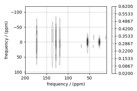
# The plot of the dataset.
levels = (np.arange(10) + 0.3) / 15  # contours are drawn at these levels.
ax = plt.subplot(projection="csdm")
cb = ax.contour(pass_data, colors="k", levels=levels, alpha=0.5, linewidths=0.5)
plt.colorbar(cb)
ax.set_xlim(200, 10)
ax.invert_yaxis()
plt.tight_layout()
plt.show()

Extract a 1D sideband intensity cross-section from the 2D dataset using the array indexing.

data1D = pass_data[1100]  # sideband dataset

# The plot of the cross-section.
ax = plt.subplot(projection="csdm")
ax.plot(data1D, color="k")
ax.invert_xaxis()
plt.tight_layout()
plt.show()

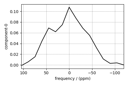
The isotropic chemical shift coordinate of the cross-section is

isotropic_shift = pass_data.x[0].coords[1100]
print(isotropic_shift)

Out:

119.8940272861969 ppm

Create a fitting model

The fitting model includes the Simulator and SignalProcessor objects. First, create the Simulator object.

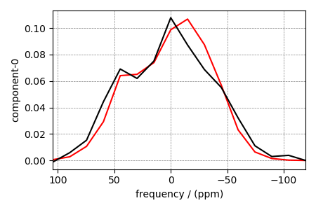
# Create the guess site and spin system for the 1D cross-section.
zeta = -70  # in ppm
eta = 0.8

site = Site(
    isotope="13C",
    isotropic_chemical_shift=0,
    shielding_symmetric={"zeta": zeta, "eta": eta},
)
spin_systems = [SpinSystem(sites=[site])]

For the sideband only cross-section, use the BlochDecaySpectrum method.

# Get the dimension information from the experiment. Note, the following function
# returns an array of two spectral dimensions corresponding to the 2D PASS dimensions.
# Use the spectral dimension that is along the anisotropic dimensions for the
# BlochDecaySpectrum method.
spectral_dims = get_spectral_dimensions(pass_data)
method = BlochDecaySpectrum(
    channels=["13C"],
    magnetic_flux_density=9.4,  # in T
    rotor_frequency=1500,  # in Hz
    spectral_dimensions=[spectral_dims[0]],
    experiment=data1D,  # also add the measurement to the method.
)

# Optimize the script by pre-setting the transition pathways for each spin system from
# the method.
for sys in spin_systems:
    sys.transition_pathways = method.get_transition_pathways(sys)

# Create the Simulator object and add the method and spin system objects.
sim = Simulator()
sim.spin_systems = spin_systems  # add the spin systems
sim.methods = [method]  # add the method
sim.run()

# Add and apply Post simulation processing.
processor = sp.SignalProcessor(operations=[sp.Scale(factor=1)])
processed_data = processor.apply_operations(data=sim.methods[0].simulation).real

# The plot of the simulation from the guess model and experiment cross-section.
ax = plt.subplot(projection="csdm")
ax.plot(processed_data, color="r", label="guess")
ax.plot(data1D, color="k", label="experiment")
ax.invert_xaxis()
plt.tight_layout()
plt.show()

Least-squares minimization with LMFIT

First, create the fitting parameters. Use the make_LMFIT_params() for a quick setup.

params = make_LMFIT_params(sim, processor)

# Fix the value of the isotropic chemical shift to zero for pure anisotropic sideband
# amplitude simulation.
params["sys_0_site_0_isotropic_chemical_shift"].vary = False
params.pretty_print()

Out:

Name                                      Value      Min      Max   Stderr     Vary     Expr Brute_Step
operation_0_Scale_factor                      1     -inf      inf     None     True     None     None
sys_0_abundance                             100        0      100     None    False      100     None
sys_0_site_0_isotropic_chemical_shift         0     -inf      inf     None    False     None     None
sys_0_site_0_shielding_symmetric_eta        0.8        0        1     None     True     None     None
sys_0_site_0_shielding_symmetric_zeta       -70     -inf      inf     None     True     None     None

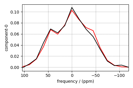
Run the minimization using LMFIT

minner = Minimizer(LMFIT_min_function, params, fcn_args=(sim, processor))
result = minner.minimize()
report_fit(result)

Out:

[[Fit Statistics]]
    # fitting method   = leastsq
    # function evals   = 25
    # data points      = 16
    # variables        = 3
    chi-square         = 2.4041e-04
    reduced chi-square = 1.8493e-05
    Akaike info crit   = -171.692083
    Bayesian info crit = -169.374317
[[Variables]]
    sys_0_site_0_isotropic_chemical_shift:  0 (fixed)
    sys_0_site_0_shielding_symmetric_zeta: -74.8435735 +/- 1.40429904 (1.88%) (init = -70)
    sys_0_site_0_shielding_symmetric_eta:   0.92016512 +/- 0.02992412 (3.25%) (init = 0.8)
    sys_0_abundance:                        100.000000 +/- 0.00000000 (0.00%) == '100'
    operation_0_Scale_factor:               1.01870585 +/- 0.02213807 (2.17%) (init = 1)
[[Correlations]] (unreported correlations are < 0.100)
    C(sys_0_site_0_shielding_symmetric_zeta, sys_0_site_0_shielding_symmetric_eta) =  0.449
    C(sys_0_site_0_shielding_symmetric_zeta, operation_0_Scale_factor)             = -0.303

Simulate the spectrum corresponding to the optimum parameters

sim.run()
processed_data = processor.apply_operations(data=sim.methods[0].simulation).real

Plot the spectrum

ax = plt.subplot(projection="csdm")
ax.plot(processed_data, color="r", label="fit")
ax.plot(data1D, color="k", label="experiment")
ax.invert_xaxis()
plt.tight_layout()
plt.show()