Note
Go to the end to download the full example code.
Extended Czjzek fitting of ¹³⁹La MAS NMR of La₀.₂Y₁.₈Si₂2O₇
The following is a demonstration on how to fit tensor distributions to an experimental spectrum using a structure-forward approach. The dataset was acquired from a sample of \(\text{La}_{0.2}\text{Y}_{1.8}\text{Si}_2\text{O}_7\) silicate glass and shared by Fernańdez-Carrioń et al. [1].
from mrsimulator import Simulator, SpinSystem, Site
from mrsimulator.method.lib import BlochDecayCTSpectrum
from mrsimulator.models import ExtCzjzekDistribution
from mrsimulator.simulator import Isotope
from mrsimulator.utils import get_spectral_dimensions
from mrsimulator import signal_processor as sp

import numpy as np
import csdmpy as cp
import lmfit
from lmfit import Minimizer
import matplotlib.pyplot as plt
Import the dataset
host = "http://ssnmr.org/sites/default/files/"
filename = "mrsimulator/La bc - LaY90 cpmg.csdf"
experiment = cp.load(host + filename).real
experiment.x[0].to("ppm", "nmr_frequency_ratio")
experiment /= experiment.max()

plt.figure(figsize=(4, 3))
ax = plt.subplot(projection="csdm")
ax.plot(experiment, "k", alpha=0.5)
plt.grid()
plt.tight_layout()
plt.show()

Calculate Noise Standard Deviation
loc = np.where(experiment.dimensions[0].coordinates < -5000e-6)
sigma = experiment[loc].std()
print(sigma)
0.006770052015781403
Setup Method and Processor
Next setup a method which simulates the experiment, again using the
get_spectral_dimensions() function to get the spectral
dimension parameters from the experimental dataset.
We also create a signal processor object which will scale the simulated spectrum.
spec_dims = get_spectral_dimensions(experiment)
method = BlochDecayCTSpectrum(
    channels=["139La"], magnetic_flux_density=17.6, spectral_dimensions=spec_dims
)

processor = sp.SignalProcessor(operations=[sp.Scale(factor=1000)])
Create a Lineshape Kernel
An approach for fitting model values to the experimental dataset could be computing the spectrum from a list of spin system objects with tensor parameters pulled from an Extended Czjzek model during each round of fitting, but this would be inefficient! The grid of \(\text{Cq}\) and \(\eta_q\) points will not change during the fit; we are interested in the probability distribution across these points.
We therefore define a function which pre-computes a lineshape kernel given a range
of \(\text{Cq}\) and \(\eta_q\) values, an NMR method, and an isotope which,
for this example, is "139La".
def make_kernel(pos, method, isotope):
    """Pre-computes the kernel to use when fitting the experimental spectrum

    Arguments:
        (np.array) pos: list of Numpy array of cq and eta points
        (Method) method: mrsimulator Method object used to simulate the spectra
        (str) isotope: Isotope of the site

    Returns:
        Lineshape kernel as a numpy array
    """
    Cq, eta = np.meshgrid(pos[0], pos[1], indexing="xy")

    spin_systems = [
        SpinSystem(sites=[Site(isotope=isotope, quadrupolar=dict(Cq=cq_, eta=e_))])
        for cq_, e_ in zip(Cq.ravel(), eta.ravel())
    ]
    sim = Simulator(spin_systems=spin_systems, methods=[method])
    sim.config.number_of_sidebands = 4
    sim.config.decompose_spectrum = "spin_system"
    sim.run(pack_as_csdm=False)  # Will return spectrum as numpy array, not CSDM object

    amp = sim.methods[0].simulation.real
    return amp.T


# Create ranges to construct cq and eta grid points
cq_range = (np.linspace(0, 100, num=100) * 0.8 + 25) * 1e6  # in Hz
eta_range = np.arange(21) / 20
pos = [cq_range, eta_range]
kernel = make_kernel(pos, method, "139La")
Make spectrum from kernel and model values
Next define a function which takes a LMFIT Parameters object, the pre-computed kernel
and a signal processor object and returns a CSDM object holding the guess spectrum.
Here the Parameters object holds attributes from the
ExtCzjzekDistribution class which is used to
create the probability density function, \({\bf f}\). Then \({\bf f}\) is
multiplied with the kernel, \({\bf K}\), to produce a spectrum, \({\bf s}\).
A constant isotropic chemical shift, whose value is also in the Parameters object, is applied to \({\bf s}\) using the Fourier shift relation. Finally, the spectrum is scaled and returned.
def make_spectrum_from_parameters(params, kernel, processor, pos, distribution):
    """Makes a spectrum with values given in a parameters object and a pre-computed
    kernel.

    Arguments:
        (Parameters) params: LMFIT Parameters object with values
        (np.array) kernel: Pre-computed spectrum kernel
        (sp.SignalProcessor) processor: SignalProcessor to apply to spectrum

    Returns:
        CSDM object of spectrum
    """
    # Extract values from parameters object
    values = params.valuesdict()
    Cq = values["dist_Cq"]
    eta = values["dist_eta"]
    eps = values["dist_eps"]
    iso_shift = values["dist_iso_shift"]

    # Setup model object and get the amplitude
    distribution.symmetric_tensor.Cq = Cq
    distribution.symmetric_tensor.eta = eta
    distribution.eps = eps
    _, _, amp = distribution.pdf(pos=pos)

    # Create spectra by dotting the amplitude distribution with the kernel
    dist = np.dot(kernel, amp.ravel())

    # Pack numpy array as csdm object and apply signal processing
    guess_dataset = cp.CSDM(
        dimensions=experiment.x,
        dependent_variables=[cp.as_dependent_variable(dist)],
    )

    # Calculate isotropic shift in Hz
    larmor_freq = Isotope(symbol="139La").gyromagnetic_ratio * 17.6
    iso_shift_in_hz = larmor_freq * iso_shift

    # Apply isotropic shift using FFT shift theorem
    guess_dataset = guess_dataset.fft()
    time_coords = guess_dataset.x[0].coordinates.value
    guess_dataset.y[0].components[0] *= np.exp(
        -np.pi * 2j * iso_shift_in_hz * time_coords
    )
    guess_dataset = guess_dataset.fft()

    # Apply signal processor and return
    processor.operations[0].factor = values["sp_scale_factor"]
    guess_dataset = processor.apply_operations(guess_dataset)
    return guess_dataset.real


def residuals(exp_spectra, simulated_spectra):
    """Returns the difference between exp_spectra and simulated_spectra"""
    return exp_spectra - simulated_spectra
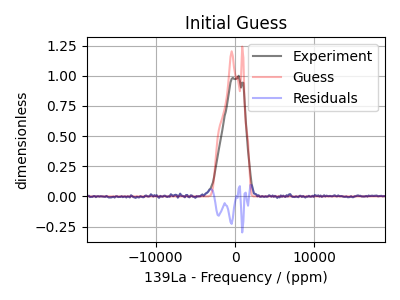
Make initial guess
Next pack the attributes to be fit into a Parameters object and plot the initial guess spectrum.
Note
If you adapt this example to your own dataset, make sure the initial guess is decently good, otherwise LMFIT is likely to fall into a local minima.
params = lmfit.Parameters()
params.add("dist_Cq", value=49.5e6)  # Hz
params.add("dist_eta", value=0.55, min=0, max=1)
params.add("dist_eps", value=0.1, min=0)
params.add("dist_iso_shift", value=350)  # ppm
params.add("sp_scale_factor", value=3.8e3, min=0)

# Plot the initial guess spectrum along with the experimental data
distribution = ExtCzjzekDistribution(
    symmetric_tensor={"Cq": params["dist_Cq"], "eta": params["dist_eta"]},
    eps=params["dist_eps"],
)
guess_distribution = distribution.pdf(pos, size=400_000, pack_as_csdm=True)

initial_guess_spectrum = make_spectrum_from_parameters(
    params, kernel, processor, pos, distribution
)
residual_spectrum = residuals(experiment, initial_guess_spectrum)

plt.figure(figsize=(4, 3))
ax = plt.subplot(projection="csdm")
ax.plot(experiment.real, "k", alpha=0.5, label="Experiment")
ax.plot(initial_guess_spectrum.real, "r", alpha=0.3, label="Guess")
ax.plot(residual_spectrum.real, "b", alpha=0.3, label="Residuals")
plt.legend()
plt.grid()
plt.title("Initial Guess")
plt.tight_layout()
plt.show()
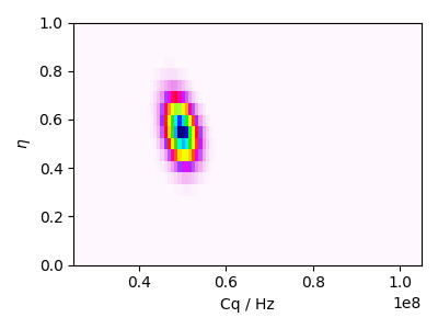
Guess distribution
plt.figure(figsize=(4, 3))
ax = plt.subplot(projection="csdm")
ax.imshow(guess_distribution, interpolation="none", cmap="gist_ncar_r", aspect="auto")
ax.set_xlabel("Cq / Hz")
ax.set_ylabel(r"$\eta$")
plt.tight_layout()
plt.show()
Least-squares minimization with LMFIT
Now define minimization function per the LMFIT specifications which will return the difference between the experimental and guess spectrum scaled by the noise standard deviation which was calculated in a previous cell.
def minimization_function(
    params, experiment, processor, kernel, pos, distribution, sigma=sigma
):
    guess_spectrum = make_spectrum_from_parameters(
        params, kernel, processor, pos, distribution
    )
    residual_spectrum = residuals(experiment, guess_spectrum)
    return residual_spectrum.y[0].components[0].real / sigma
Sinice the probabilty distribution is generated from a sparsely sampled from a 5D second rank tensor parameter space, we increase the diff_step size from machine precession to avoid approaching local minima from noise.
scipy_minimization_kwargs = dict(
    diff_step=1e-4,  # Increase step size from machine precession
    gtol=1e-10,  # Decrease global convergence requirement (default 1e-8)
    xtol=1e-10,  # Decrease variable convergence requirement (default 1e-8)
    verbose=2,  # Print minimization info during each step
    loss="linear",
)

minner = Minimizer(
    minimization_function,
    params,
    fcn_args=(experiment, processor, kernel, pos, distribution),
    **scipy_minimization_kwargs,
)
result = minner.minimize(method="least_squares")
best_fit_params = result.params  # Grab the Parameters object from the best fit
result
   Iteration     Total nfev        Cost      Cost reduction    Step norm     Optimality
       0              1         5.6230e+03                                    6.24e+04
       1              2         6.4862e+02      4.97e+03       9.22e+04       1.21e+04
       2              3         2.1067e+02      4.38e+02       1.90e+05       1.76e+03
       3              4         1.7648e+02      3.42e+01       2.80e+05       6.48e+02
       4              5         1.7448e+02      1.99e+00       2.47e+04       4.81e+02
       5              6         1.7404e+02      4.42e-01       5.66e+04       5.70e+01
       6              7         1.7399e+02      4.59e-02       1.51e+03       9.68e+01
       7             19         1.7399e+02      0.00e+00       0.00e+00       9.68e+01
`xtol` termination condition is satisfied.
Function evaluations 19, initial cost 5.6230e+03, final cost 1.7399e+02, first-order optimality 9.68e+01.
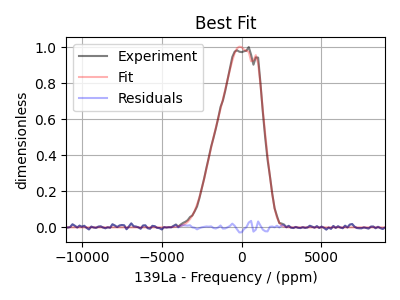
Plot the best-fit solution
Finally, plot the best fit spectrum and the residuals.
final_fit = make_spectrum_from_parameters(
    best_fit_params, kernel, processor, pos, distribution
)
residual_spectrum = residuals(experiment, final_fit)

plt.figure(figsize=(4, 3))
ax = plt.subplot(projection="csdm")
ax.plot(experiment, "k", alpha=0.5, label="Experiment")
ax.plot(final_fit, "r", alpha=0.3, label="Fit")
ax.plot(residual_spectrum, "b", alpha=0.3, label="Residuals")
plt.legend()
ax.set_xlim(-11000, 9000)
plt.grid()
plt.title("Best Fit")
plt.tight_layout()
plt.show()
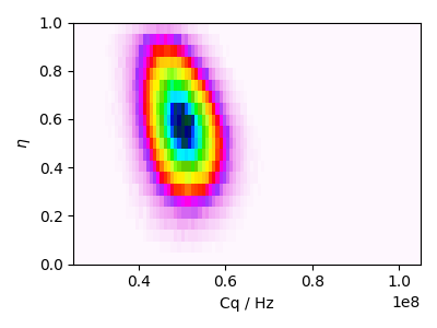
Best fit probability distribution
prob = distribution.pdf(pos, pack_as_csdm=True)
plt.figure(figsize=(4, 3))
ax = plt.subplot(projection="csdm")
ax.imshow(prob, interpolation="none", cmap="gist_ncar_r", aspect="auto")
ax.set_xlabel("Cq / Hz")
ax.set_ylabel(r"$\eta$")
plt.tight_layout()
plt.show()
Total running time of the script: (0 minutes 3.504 seconds)