Note
Go to the end to download the full example code.
Fitting a Czjzek Model
In this example, we illustrate an application of mrsimulator in fitting a lineshape from a Czjzek distribution of quadrupolar tensors to an experimental \(^{27}\text{Al}\) MAS spectrum of a phospho-aluminosilicate glass. Setting up the least-squares minimization for a distribution of spin systems is slightly different than that of a crystalline solid.
- There are 4 steps involved in the processs:
Importing the experimental dataset,
Generating a pre-computed line shape kernel of subspectra,
Creating parameters for the Czjzek distribution model from an initial guess,
Minimizing and visualizing.
import numpy as np
import csdmpy as cp
import matplotlib.pyplot as plt
import mrsimulator.signal_processor as sp
from mrsimulator.simulator.config import ConfigSimulator
import mrsimulator.utils.spectral_fitting as sf
from lmfit import Minimizer

from mrsimulator.method.lib import BlochDecayCTSpectrum
from mrsimulator.utils import get_spectral_dimensions

from mrsimulator.models.czjzek import CzjzekDistribution
from mrsimulator.models.utils import LineShapeKernel
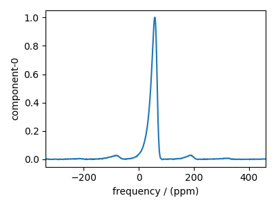
Import the experimental dataset
Below we import and visualize the experimental dataset.
host = "http://ssnmr.org/sites/default/files/mrsimulator/"
filename = "20K_20Al_10P_50Si_HahnEcho_27Al.csdf"
exp_data = cp.load(host + filename).real

exp_data.x[0].to("ppm", "nmr_frequency_ratio")
exp_data /= exp_data.max()

plt.figure(figsize=(4, 3))
ax = plt.subplot(projection="csdm")
ax.plot(exp_data)
plt.tight_layout()
plt.show()
Generating a line shape kernel
The Czjzek distribution is a statistical model that represents a five-dimensional multivariate normal distribution of second-rank tensor components. These random second-rank tensors are converted into corresponding anisotropy and asymmetry parameters using the Haeberlen convention. The resulting parameters are then binned on a two-dimensional grid, forming the Czjzek probability distribution. The Czjzek spectra is which are the probability weighted sum of lineshapes at each grid point.
However, simulating the spectra of spin systems at each minimization step for the least-squares fitting is computationally expensive. A more efficient way is to pre-define a grid system for the tensor parameters, simulate a library of sub-spectra for each grid point, and only update the probability distribution during each minimization step.
To simulate the spectra of the given experiment, we create a Method object. Using this method, we generate a kernel of lineshape sub-spectra defined on a polar grid by using the LineShapeKernel class. The argument “method” is the mrsimulator method object used for the simulation, “pos” is a tuple of coordinates defining the two-dimensional grid, “polar” defines a polar parameter coordinate space, and “config” is the Simulator config object used in lineshape simulation. Here, we use the “config” argument to set the number of sidebands as 8.
The kernel is generated with the “generate_lineshape()” function, where we pass the “tensor_type=’quadrupolar’” argument to specify a quadrupolar parameter grid. A symmetric shielding lineshape kernel can also be generated by specifying
# Create a Method object to simulate the spectrum
spectral_dimensions = get_spectral_dimensions(exp_data)
method = BlochDecayCTSpectrum(
    channels=["27Al"],
    rotor_frequency=14.2e3,
    spectral_dimensions=spectral_dimensions,
    experiment=exp_data,
)

# Define a polar grid for the lineshape kernel
x = np.linspace(0, 2e7, num=36)
y = np.linspace(0, 2e7, num=36)
pos = (x, y)

# Generate the kernel
sim_config = ConfigSimulator(number_of_sidebands=8)
quad_kernel = LineShapeKernel(method=method, pos=pos, polar=True, config=sim_config)
quad_kernel.generate_lineshape(tensor_type="quadrupolar")

print("Desired Kernel shape: ", (x.size * y.size, spectral_dimensions[0]["count"]))
print("Actual Kernel shape:  ", quad_kernel.kernel.shape)
Desired Kernel shape:  (1296, 512)
Actual Kernel shape:   (1296, 512)
Create a Parameters object
Next, we create an instance of the CzjzekDistribution class with initial guess values along with a SignalProcessor object.
# Create initial guess CzjzekDistribution
cz_model = CzjzekDistribution(
    mean_isotropic_chemical_shift=60.0, sigma=1.4e6, polar=True
)
all_models = [cz_model]

processor = sp.SignalProcessor(
    operations=[
        sp.IFFT(),
        sp.apodization.Gaussian(FWHM="600 Hz"),
        sp.FFT(),
        sp.Scale(factor=0.3),
    ]
)
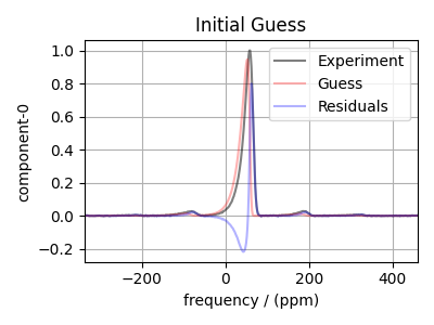
Make the Parameters object and simulate a guess spectrum. Note that the variable sf_kwargs holds some additional keyword arguments that many of the spectral fitting function takes in. This dictionary needs to be updated to reflect any changes made in the minimization.
params = sf.make_LMFIT_params(spin_system_models=all_models, processors=[processor])

# Additional keyword arguments passed to best-fit and residual functions.
sf_kwargs = dict(
    kernel=quad_kernel,
    spin_system_models=all_models,
    processor=processor,
)

# Make a guess and residuals spectrum from the initial guess
guess = sf.bestfit_dist(params=params, **sf_kwargs)
residuals = sf.residuals_dist(params=params, **sf_kwargs)

plt.figure(figsize=(4, 3))
ax = plt.subplot(projection="csdm")
ax.plot(exp_data, "k", alpha=0.5, label="Experiment")
ax.plot(guess, "r", alpha=0.3, label="Guess")
ax.plot(residuals, "b", alpha=0.3, label="Residuals")
plt.legend()
plt.grid()
plt.title("Initial Guess")
plt.tight_layout()
plt.show()

# Print the Parameters object
params
Create and run a minimization
Finally, a Minimizer object is created and a minimization run using least-squares. The same arguments defined in the addtl_sf_kwargs variable are also passed to the minimizer. Sinice the probabilty distribution is generated from a sparsely sampled from a 5D second rank tensor parameter space, we increase the diff_step size from machine precession to avoid approaching local minima from noise.
scipy_minimization_kwargs = dict(
    diff_step=1e-4,  # Increase step size from machine precesion.
    gtol=1e-10,  # Decrease global convergence requirement (default 1e-8)
    xtol=1e-10,  # Decrease variable convergence requirement (default 1e-8)
    verbose=2,  # Print minimization info during each step
    loss="linear",
)

minner = Minimizer(
    sf.LMFIT_min_function_dist,
    params,
    fcn_kws=sf_kwargs,
    **scipy_minimization_kwargs,
)
result = minner.minimize(method="least_squares")
result
   Iteration     Total nfev        Cost      Cost reduction    Step norm     Optimality
       0              1         1.9247e+00                                    4.13e+00
       1              2         4.6728e-01      1.46e+00       9.95e+04       5.99e+00
       2              3         8.6644e-02      3.81e-01       5.92e+04       6.13e-01
       3              4         1.3243e-02      7.34e-02       2.66e+03       4.29e-01
       4              5         6.4638e-03      6.78e-03       4.67e+04       2.84e-02
       5              6         6.4205e-03      4.32e-05       4.89e+03       1.23e-03
       6              7         6.4204e-03      7.48e-08       6.57e+01       6.89e-06
       7              8         6.4204e-03      4.37e-10       6.95e+00       4.08e-06
       8             15         6.4204e-03      0.00e+00       0.00e+00       4.08e-06
`xtol` termination condition is satisfied.
Function evaluations 15, initial cost 1.9247e+00, final cost 6.4204e-03, first-order optimality 4.08e-06.
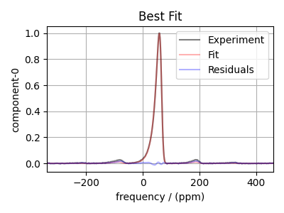
Plot the best-fit spectrum
bestfit = sf.bestfit_dist(params=result.params, **sf_kwargs)
residuals = sf.residuals_dist(params=result.params, **sf_kwargs)

plt.figure(figsize=(4, 3))
ax = plt.subplot(projection="csdm")
ax.plot(exp_data, "k", alpha=0.5, label="Experiment")
ax.plot(bestfit, "r", alpha=0.3, label="Fit")
ax.plot(residuals, "b", alpha=0.3, label="Residuals")
plt.legend()
plt.grid()
plt.title("Best Fit")
plt.tight_layout()
plt.show()
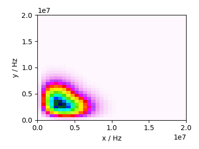
Plot the best-fit distribution
for i, model in enumerate(all_models):
    model.update_lmfit_params(result.params, i)

amp = cz_model.pdf(pos=pos, pack_as_csdm=True)

plt.figure(figsize=(4, 3))
ax = plt.subplot(projection="csdm")
ax.imshow(amp, cmap="gist_ncar_r", interpolation="none", aspect="auto")
ax.set_xlabel("x / Hz")
ax.set_ylabel("y / Hz")
plt.tight_layout()
plt.show()
Total running time of the script: (0 minutes 2.997 seconds)