Note
Go to the end to download the full example code.
⁸⁷Rb 2D QMAT NMR of Rb₂SO₄
The following is an illustration for fitting 2D QMAT/QPASS datasets. The example dataset is a \(^{87}\text{Rb}\) 2D QMAT spectrum of \(\text{Rb}_2\text{SO}_4\) from Walder et al. [1]
import numpy as np
import csdmpy as cp
import matplotlib.pyplot as plt
from lmfit import Minimizer

from mrsimulator import Simulator, SpinSystem, Site
from mrsimulator.method.lib import SSB2D
from mrsimulator import signal_processor as sp
from mrsimulator.utils import spectral_fitting as sf
from mrsimulator.utils import get_spectral_dimensions
from mrsimulator.spin_system.tensors import SymmetricTensor
Import the dataset
filename = "https://ssnmr.org/sites/default/files/mrsimulator/Rb2SO4_QMAT.csdf"
qmat_dataset = cp.load(filename)
# For the spectral fitting, we only focus on the real part of the complex dataset.
qmat_dataset = qmat_dataset.real
# Convert the coordinates along each dimension from Hz to ppm.
_ = [item.to("ppm", "nmr_frequency_ratio") for item in qmat_dataset.dimensions]
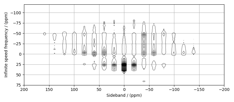
# plot of the dataset.
max_amp = qmat_dataset.max()
levels = (np.arange(31) + 0.15) * max_amp / 32 # contours are drawn at these levels.
options = dict(levels=levels, alpha=1, linewidths=0.5) # plot options
plt.figure(figsize=(8, 3.5))
ax = plt.subplot(projection="csdm")
ax.contour(qmat_dataset.T, colors="k", **options)
ax.set_xlim(200, -200)
ax.set_ylim(75, -120)
plt.grid()
plt.tight_layout()
plt.show()
Estimate noise statistics from the dataset
noise_region = np.where(qmat_dataset.dimensions[0].coordinates < -175e-6)
noise_data = qmat_dataset[noise_region]

plt.figure(figsize=(3.75, 2.5))
ax = plt.subplot(projection="csdm")
ax.imshow(noise_data.T, aspect="auto", interpolation="none")
plt.title("Noise section")
plt.axis("off")
plt.tight_layout()
plt.show()

noise_mean, sigma = noise_data.mean(), noise_data.std()
noise_mean, sigma
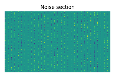
(<Quantity 0.02628929>, <Quantity 3.0965025>)
Create a fitting model
Guess model
Create a guess list of spin systems.
Rb_1 = Site(
    isotope="87Rb",
    isotropic_chemical_shift=16,  # in ppm
    quadrupolar=SymmetricTensor(Cq=5.3e6, eta=0.1),  # Cq in Hz
)
Rb_2 = Site(
    isotope="87Rb",
    isotropic_chemical_shift=40,  # in ppm
    quadrupolar=SymmetricTensor(Cq=2.2e6, eta=0.95),  # Cq in Hz
)

spin_systems = [SpinSystem(sites=[s]) for s in [Rb_1, Rb_2]]
Method
Create the SSB2D method.
# Get the spectral dimension parameters from the experiment.
spectral_dims = get_spectral_dimensions(qmat_dataset)

PASS = SSB2D(
    channels=["87Rb"],
    magnetic_flux_density=9.395,  # in T
    rotor_frequency=2604,  # in Hz
    spectral_dimensions=spectral_dims,
    experiment=qmat_dataset,  # add the measurement to the method.
)
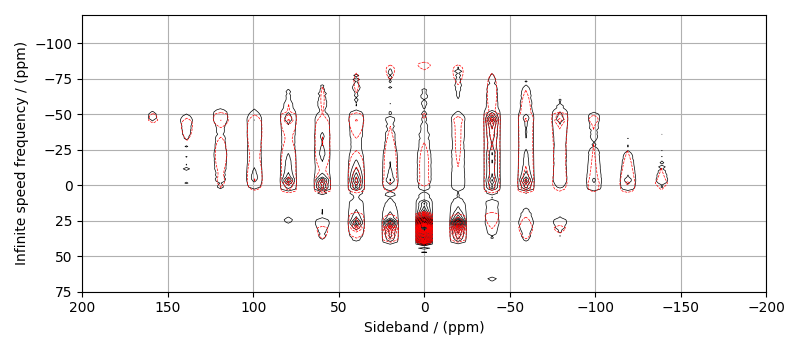
Guess Spectrum
# Simulation
# ----------
sim = Simulator(spin_systems=spin_systems, methods=[PASS])
sim.run()

# Post Simulation Processing
# --------------------------
processor = sp.SignalProcessor(
    operations=[
        # Lorentzian convolution along the isotropic dimensions.
        sp.FFT(dim_index=0),
        sp.apodization.Gaussian(FWHM="100 Hz"),
        sp.IFFT(dim_index=0),
        sp.Scale(factor=1e8),
    ]
)
processed_dataset = processor.apply_operations(dataset=sim.methods[0].simulation).real

# Plot of the guess Spectrum
# --------------------------
plt.figure(figsize=(8, 3.5))
ax = plt.subplot(projection="csdm")
ax.contour(qmat_dataset.T, colors="k", **options)
ax.contour(processed_dataset.T, colors="r", linestyles="--", **options)
ax.set_xlim(200, -200)
ax.set_ylim(75, -120)
plt.grid()
plt.tight_layout()
plt.show()
Least-squares minimization with LMFIT
Use the make_LMFIT_params() for a quick
setup of the fitting parameters.
params = sf.make_LMFIT_params(sim, processor)
params["SP_0_operation_1_Gaussian_FWHM"].min = 0
print(params.pretty_print(columns=["value", "min", "max", "vary", "expr"]))
Name                                      Value      Min      Max     Vary     Expr
SP_0_operation_1_Gaussian_FWHM              100        0      inf     True     None
SP_0_operation_3_Scale_factor             1e+08     -inf      inf     True     None
sys_0_abundance                              50        0      100     True     None
sys_0_site_0_isotropic_chemical_shift        16     -inf      inf     True     None
sys_0_site_0_quadrupolar_Cq             5.3e+06     -inf      inf     True     None
sys_0_site_0_quadrupolar_eta                0.1        0        1     True     None
sys_1_abundance                              50        0      100    False 100-sys_0_abundance
sys_1_site_0_isotropic_chemical_shift        40     -inf      inf     True     None
sys_1_site_0_quadrupolar_Cq             2.2e+06     -inf      inf     True     None
sys_1_site_0_quadrupolar_eta               0.95        0        1     True     None
None
Solve the minimizer using LMFIT
opt = sim.optimize()  # Pre-compute transition pathways
minner = Minimizer(
    sf.LMFIT_min_function,
    params,
    fcn_args=(sim, processor, sigma),
    fcn_kws={"opt": opt},
)
result = minner.minimize()
result
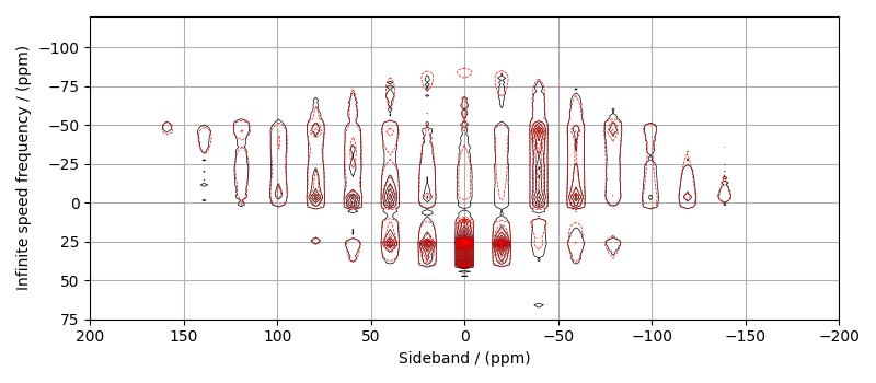
The best fit solution
best_fit = sf.bestfit(sim, processor)[0].real

# Plot of the best fit solution
plt.figure(figsize=(8, 3.5))
ax = plt.subplot(projection="csdm")
ax.contour(qmat_dataset.T, colors="k", **options)
ax.contour(best_fit.T, colors="r", linestyles="--", **options)
ax.set_xlim(200, -200)
ax.set_ylim(75, -120)
plt.grid()
plt.tight_layout()
plt.show()
Total running time of the script: (0 minutes 7.217 seconds)