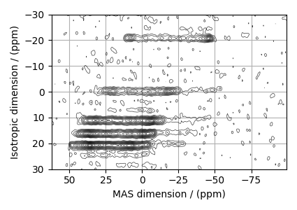
¹⁷O 2D DAS NMR of Coesite

Coesite is a high-pressure (2-3 GPa) and high-temperature (700°C) polymorph of silicon dioxide \(\text{SiO}_2\). Coesite has five crystallographic \(^{17}\text{O}\) sites. The experimental dataset used in this example is published in Grandinetti et al. [1]

import numpy as np
import csdmpy as cp
import matplotlib.pyplot as plt
from lmfit import Minimizer

from mrsimulator import Simulator
from mrsimulator import signal_processor as sp
from mrsimulator.utils import spectral_fitting as sf
from mrsimulator.utils import get_spectral_dimensions
from mrsimulator.utils.collection import single_site_system_generator
from mrsimulator.method import Method, SpectralDimension, SpectralEvent, MixingEvent

Import the dataset

filename = "https://ssnmr.org/sites/default/files/mrsimulator/DASCoesite.csdf"
experiment = cp.load(filename)

# For spectral fitting, we only focus on the real part of the complex dataset
experiment = experiment.real

# Convert the coordinates along each dimension from Hz to ppm.
_ = [item.to("ppm", "nmr_frequency_ratio") for item in experiment.dimensions]

# plot of the dataset.
max_amp = experiment.max()
levels = (np.arange(14) + 1) * max_amp / 15  # contours are drawn at these levels.
options = dict(levels=levels, alpha=0.75, linewidths=0.5)  # plot options

plt.figure(figsize=(4.25, 3.0))
ax = plt.subplot(projection="csdm")
ax.contour(experiment, colors="k", **options)
ax.invert_xaxis()
ax.set_ylim(30, -30)
plt.grid()
plt.tight_layout()
plt.show()

Estimate noise statistics from the dataset

coords = experiment.dimensions[0].coordinates
noise_region = np.where(coords < -75e-6)
noise_data = experiment[noise_region]

plt.figure(figsize=(3.75, 2.5))
ax = plt.subplot(projection="csdm")
ax.imshow(noise_data, aspect="auto", interpolation="none")
plt.title("Noise section")
plt.axis("off")
plt.tight_layout()
plt.show()

noise_mean, sigma = noise_data.mean(), noise_data.std()
noise_mean, sigma

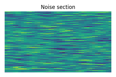
(<Quantity -21.397367>, <Quantity 970.9593>)

Create a fitting model

Guess model

Create a guess list of spin systems.

shifts = [29, 39, 54.8, 51, 56]  # in ppm
Cq = [6.1e6, 5.4e6, 5.5e6, 5.5e6, 5.1e6]  # in  Hz
eta = [0.1, 0.2, 0.15, 0.15, 0.3]
abundance_ratio = [1, 1, 2, 2, 2]
abundance = np.asarray(abundance_ratio) / 8 * 100  # in %

spin_systems = single_site_system_generator(
    isotope="17O",
    isotropic_chemical_shift=shifts,
    quadrupolar={"Cq": Cq, "eta": eta},
    abundance=abundance,
)

Method

Create the DAS method.

# Get the spectral dimension parameters from the experiment.
spectral_dims = get_spectral_dimensions(experiment)

DAS = Method(
    channels=["17O"],
    magnetic_flux_density=11.744,  # in T
    rotor_frequency=np.inf,
    spectral_dimensions=[
        SpectralDimension(
            **spectral_dims[0],
            events=[
                SpectralEvent(
                    fraction=0.5,
                    rotor_angle=37.38 * np.pi / 180,  # in rads
                    transition_queries=[{"ch1": {"P": [-1], "D": [0]}}],
                ),
                MixingEvent(query="NoMixing"),
                SpectralEvent(
                    fraction=0.5,
                    rotor_angle=79.19 * np.pi / 180,  # in rads
                    transition_queries=[{"ch1": {"P": [-1], "D": [0]}}],
                ),
                MixingEvent(query="NoMixing"),
            ],
        ),
        # The last spectral dimension block is the direct-dimension
        SpectralDimension(
            **spectral_dims[1],
            events=[
                SpectralEvent(
                    rotor_angle=54.735 * np.pi / 180,  # in rads
                    transition_queries=[{"ch1": {"P": [-1], "D": [0]}}],
                )
            ],
        ),
    ],
    experiment=experiment,  # also add the measurement to the method.
)

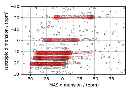
Guess Spectrum

# Simulation
# ----------
sim = Simulator(spin_systems=spin_systems, methods=[DAS])
sim.config.number_of_sidebands = 1  # no sidebands are required for this dataset.
sim.run()

# Post Simulation Processing
# --------------------------
processor = sp.SignalProcessor(
    operations=[
        # Gaussian convolution along both dimensions.
        sp.IFFT(dim_index=(0, 1)),
        sp.apodization.Gaussian(FWHM="0.15 kHz", dim_index=0),
        sp.apodization.Gaussian(FWHM="0.1 kHz", dim_index=1),
        sp.FFT(dim_index=(0, 1)),
        sp.Scale(factor=4e8),
    ]
)
processed_dataset = processor.apply_operations(dataset=sim.methods[0].simulation).real

# Plot of the guess Spectrum
# --------------------------
plt.figure(figsize=(4.25, 3.0))
ax = plt.subplot(projection="csdm")
ax.contour(experiment, colors="k", **options)
ax.contour(processed_dataset, colors="r", linestyles="--", **options)
ax.invert_xaxis()
ax.set_ylim(30, -30)
plt.grid()
plt.tight_layout()
plt.show()

Least-squares minimization with LMFIT

Use the make_LMFIT_params() for a quick setup of the fitting parameters.

params = sf.make_LMFIT_params(sim, processor)
print(params.pretty_print(columns=["value", "min", "max", "vary", "expr"]))

Name                                      Value      Min      Max     Vary     Expr
SP_0_operation_1_Gaussian_FWHM             0.15     -inf      inf     True     None
SP_0_operation_2_Gaussian_FWHM              0.1     -inf      inf     True     None
SP_0_operation_4_Scale_factor             4e+08     -inf      inf     True     None
sys_0_abundance                            12.5        0      100     True     None
sys_0_site_0_isotropic_chemical_shift        29     -inf      inf     True     None
sys_0_site_0_quadrupolar_Cq             6.1e+06     -inf      inf     True     None
sys_0_site_0_quadrupolar_eta                0.1        0        1     True     None
sys_1_abundance                            12.5        0      100     True     None
sys_1_site_0_isotropic_chemical_shift        39     -inf      inf     True     None
sys_1_site_0_quadrupolar_Cq             5.4e+06     -inf      inf     True     None
sys_1_site_0_quadrupolar_eta                0.2        0        1     True     None
sys_2_abundance                              25        0      100     True     None
sys_2_site_0_isotropic_chemical_shift      54.8     -inf      inf     True     None
sys_2_site_0_quadrupolar_Cq             5.5e+06     -inf      inf     True     None
sys_2_site_0_quadrupolar_eta               0.15        0        1     True     None
sys_3_abundance                              25        0      100     True     None
sys_3_site_0_isotropic_chemical_shift        51     -inf      inf     True     None
sys_3_site_0_quadrupolar_Cq             5.5e+06     -inf      inf     True     None
sys_3_site_0_quadrupolar_eta               0.15        0        1     True     None
sys_4_abundance                              25        0      100    False 100-sys_0_abundance-sys_1_abundance-sys_2_abundance-sys_3_abundance
sys_4_site_0_isotropic_chemical_shift        56     -inf      inf     True     None
sys_4_site_0_quadrupolar_Cq             5.1e+06     -inf      inf     True     None
sys_4_site_0_quadrupolar_eta                0.3        0        1     True     None
None

Solve the minimizer using LMFIT

opt = sim.optimize()  # Pre-compute transition pathways
minner = Minimizer(
    sf.LMFIT_min_function,
    params,
    fcn_args=(sim, processor, sigma),
    fcn_kws={"opt": opt},
)
result = minner.minimize(method="powell")
result

Fit Result

Fit Statistics

fitting method	Powell
# function evals	2049
# data points	131072
# variables	22
chi-square	168600.804
reduced chi-square	1.28653799
Akaike info crit.	33046.2285
Bayesian info crit.	33261.4655

Parameters

name	value	initial value	min	max	vary	expression
sys_0_site_0_isotropic_chemical_shift	27.8052443	29.0	-inf	inf	True
sys_0_site_0_quadrupolar_Cq	6099804.83	6100000.0	-inf	inf	True
sys_0_site_0_quadrupolar_eta	0.01098461	0.1	0.00000000	1.00000000	True
sys_0_abundance	11.1490760	12.5	0.00000000	100.000000	True
sys_1_site_0_isotropic_chemical_shift	38.5407557	39.0	-inf	inf	True
sys_1_site_0_quadrupolar_Cq	5399540.11	5400000.0	-inf	inf	True
sys_1_site_0_quadrupolar_eta	0.19999325	0.2	0.00000000	1.00000000	True
sys_1_abundance	13.9139575	12.5	0.00000000	100.000000	True
sys_2_site_0_isotropic_chemical_shift	55.9053247	54.8	-inf	inf	True
sys_2_site_0_quadrupolar_Cq	5500748.93	5500000.0	-inf	inf	True
sys_2_site_0_quadrupolar_eta	0.15000793	0.15	0.00000000	1.00000000	True
sys_2_abundance	24.6417749	25.0	0.00000000	100.000000	True
sys_3_site_0_isotropic_chemical_shift	51.2703228	51.0	-inf	inf	True
sys_3_site_0_quadrupolar_Cq	5499820.53	5500000.0	-inf	inf	True
sys_3_site_0_quadrupolar_eta	0.20955504	0.15	0.00000000	1.00000000	True
sys_3_abundance	23.7048271	25.0	0.00000000	100.000000	True
sys_4_site_0_isotropic_chemical_shift	55.6923606	56.0	-inf	inf	True
sys_4_site_0_quadrupolar_Cq	5100001.54	5100000.0	-inf	inf	True
sys_4_site_0_quadrupolar_eta	0.30000019	0.3	0.00000000	1.00000000	True
sys_4_abundance	26.5903644	25.0	0.00000000	100.000000	False	100-sys_0_abundance-sys_1_abundance-sys_2_abundance-sys_3_abundance
SP_0_operation_1_Gaussian_FWHM	0.36249298	0.15	-inf	inf	True
SP_0_operation_2_Gaussian_FWHM	0.13853213	0.1	-inf	inf	True
SP_0_operation_4_Scale_factor	4.0188e+08	400000000.0	-inf	inf	True

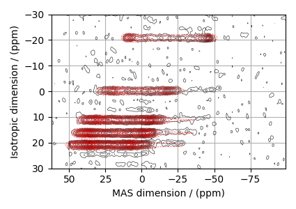
The best fit solution

best_fit = sf.bestfit(sim, processor)[0].real

# Plot the spectrum
plt.figure(figsize=(4.25, 3.0))
ax = plt.subplot(projection="csdm")
ax.contour(experiment, colors="k", **options)
ax.contour(best_fit, colors="r", linestyles="--", **options)
ax.invert_xaxis()
ax.set_ylim(30, -30)
plt.grid()
plt.tight_layout()
plt.show()

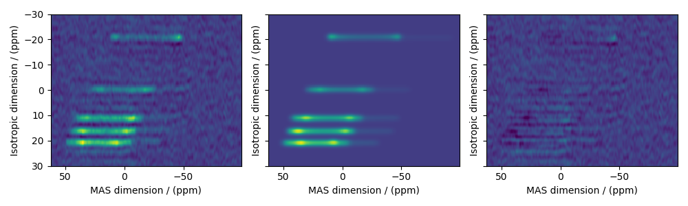
The best fit solution

residuals = sf.residuals(sim, processor)[0].real

fig, ax = plt.subplots(
    1, 3, sharey=True, figsize=(10, 3.0), subplot_kw={"projection": "csdm"}
)
vmax, vmin = experiment.max(), experiment.min()
for i, dat in enumerate([experiment, best_fit, residuals]):
    ax[i].imshow(dat, aspect="auto", vmax=vmax, vmin=vmin, interpolation="none")
    ax[i].invert_xaxis()
ax[0].set_ylim(30, -30)
plt.tight_layout()
plt.show()

[1]

Grandinetti, P. J., Baltisberger, J. H., Farnan, I., Stebbins, J. F., Werner, U. and Pines, A. Solid-State \(^{17}\text{O}\) Magic-Angle and Dynamic-Angle Spinning NMR Study of the \(\text{SiO}_2\) Polymorph Coesite, J. Phys. Chem. 1995, 99, 32, 12341-12348. DOI: 10.1021/j100032a045