Czjzek distribution
The Czjzek distribution models random variations of second-rank traceless symmetric tensors about zero, i.e., a tensor with zeta of zero. An analytical expression for the Czjzek distribution exists (cite), which follows
where \(\zeta\) and \(\eta\) are the Haberlen components of the tensor and \(\sigma\) is the Czjzek width parameter. See Czjzek distribution for a further mathematical description of the model.
The remainder of this page quickly describes how to generate Czjzek distributions and generate
SpinSystem instances from these distributions. Also, look at the
gallery examples using the Czjzek distribution listed at the bottom of this page.
Creating and sampling a Czjzek distribution
To generate a Czjzek distribution, use the CzjzekDistribution
class as follows.
from mrsimulator.models import CzjzekDistribution

cz_model = CzjzekDistribution(sigma=0.8)
The CzjzekDistribution class accepts the argument, sigma, which is the standard
deviation of the second-rank traceless symmetric tensor parameters. In the above example,
we create cz_model as an instance of the CzjzekDistribution class with
\(\sigma=0.8\).
Note, cz_model is only a class instance of the Czjzek distribution. You can either
draw random points from this distribution or generate a probability distribution
function. Let’s first draw points from this distribution, using the
rvs() method of the instance.
zeta_dist, eta_dist = cz_model.rvs(size=50000)
In the above example, we draw 50000 random points of the distribution. The output zeta_dist and eta_dist hold the tensor parameter coordinates of the points, defined in the Haeberlen convention. It is further assumed that the points in zeta_dist are in units of ppm while eta_dist has values since \(\eta\) is dimensionless. The scatter plot of these coordinates is shown below.
import matplotlib.pyplot as plt

plt.scatter(zeta_dist, eta_dist, s=4, alpha=0.02)
plt.xlabel("$\\zeta$ / ppm")
plt.ylabel("$\\eta$")
plt.xlim(-15, 15)
plt.ylim(0, 1)
plt.tight_layout()
plt.show()
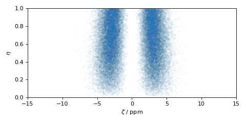
Figure 10 Random sampling of Czjzek distribution of shielding tensors.
Creating and sampling a Czjzek distribution in polar coordinates
The CzjzekDistribution class also supports sampling tensors in polar coordinates. The logic behind transforming from a \(\zeta\)-\(\eta\) Cartesian grid is further described in mrinversion (cite), and the following definitions are used
Because Cartesian grids are more manageable in computation, the above polar piece-wise grid is re-expressed as the x-y Cartesian grid following,
Below, we create another instance of the CzjzekDistribution
class with the same value of \(sigma=0.8\), but we now also include the argument polar=True
which means the rvs() will sample x and y points.
cz_model_polar = CzjzekDistribution(sigma=0.8, polar=True)

# Sample (x, y) points
x_dist, y_dist = cz_model_polar.rvs(size=50000)

# Plot the distribution
plt.figure(figsize=(4, 4))
plt.scatter(x_dist, y_dist, s=4, alpha=0.02)
plt.xlabel("$x$ / ppm")
plt.ylabel("$y$ / ppm")
plt.xlim(0, 8)
plt.ylim(0, 8)
plt.tight_layout()
plt.show()
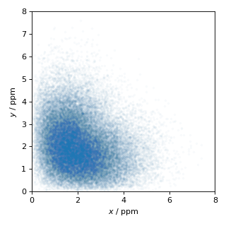
Figure 12 Random sampling of Czjzek distribution of shielding tensors in polar coordinates.
Generating probability distribution functions from a Czjzek model
The pdf() instance method will generate a
probability distribution function on the supplied grid using the analytical function defined above.
The provided grid – passed to the pos keyword argument – needs to be defined in either
Cartesian or polar coordinates, depending on whether the
polar attribute is True or False.
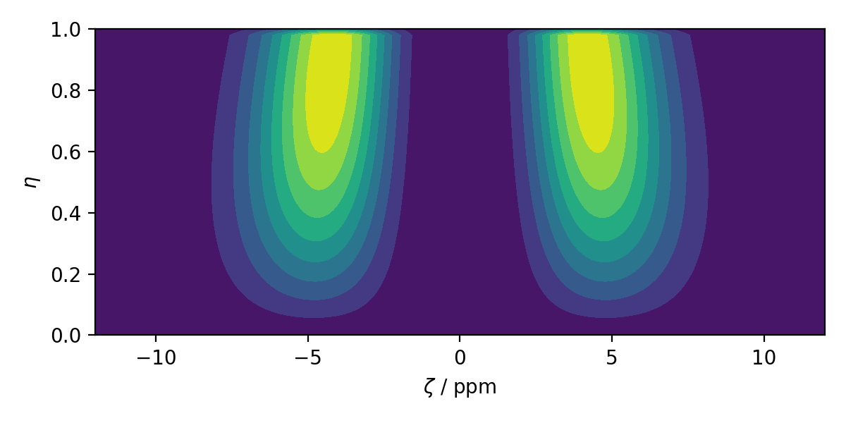
Below, we generate and plot a probability distribution on a \(\zeta\)-\(\eta\) Cartesian
grid where zeta_range and eta_range define the desired coordinates in each dimension of thes
grid system.
import numpy as np

cz_model = CzjzekDistribution(sigma=1.2, polar=False)  # sample in (zeta, eta)

zeta_range = np.linspace(-12, 12, num=200)  # pre-defined zeta range in units of ppm
eta_range = np.linspace(0, 1, num=50)       # pre-defined eta range.
zeta_grid, eta_grid, amp = cz_model.pdf(pos=[zeta_range, eta_range])
Here, zeta_grid and eta_grid are numpy arrays defining a set of pair-wise points on the
grid system, and amp is another numpy array holding the probability density at each point
on the grid. Below, the distribution is plotted
plt.contourf(zeta_grid, eta_grid, amp, levels=10)
plt.xlabel("$\\zeta$ / ppm")
plt.ylabel("$\\eta$")
plt.tight_layout()
plt.show()
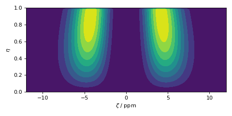
Figure 14 Czjzek Distribution of shielding tensors.
—
The probability distribution function can also be generated in polar coordinates. The workflow
is the same, except we now define an (x, y) grid system using the variables x_range
and y_range. The code to generate and plot the polar Czjzek distribution is shown below.
cz_model_polar = CzjzekDistribution(sigma=1.2, polar=True)  # sample in (x, y)

x_range = np.linspace(0, 10, num=150)
y_range = np.linspace(0, 10, num=150)
x_grid, y_grid, amp = cz_model_polar.pdf(pos=[x_range, y_range])

plt.figure(figsize=(4, 4))
plt.contourf(x_grid, y_grid, amp, levels=10)
plt.xlabel("$x$ / ppm")
plt.ylabel("$y$ / ppm")
plt.tight_layout()
plt.show()
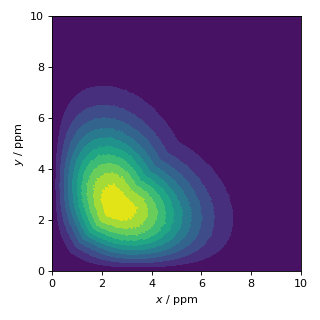
Figure 16 Czjzek Distribution of shielding tensors in polar coordinates.
Distributions of shielding and quadrupolar tensors and a note on units
The CzjzekDistribution class can be used to generate
distributions for both symmetric chemical shielding tensors and electric field gradient
tensors. It is important to note the Czjzek model is only aware of the Haberlen components
of the tensors and not the units of the tensor. In the above code cells, we generated
distributions for symmetric shielding tensors and assumed all units for \(\zeta\) were
in ppm.
Quadrupolar tensors, defined using values of \(C_q\) in MHz and unitless \(\eta\), can also be drawn from the Czjzek distribution in the same manner; however, the dimensions are assumed to be in units of MHz. The following code draws a distribution of quadrupolar tensor parameters.
Cq_range = np.linspace(-12, 12, num=200)  # pre-defined Cq range in units of MHz
eta_range = np.linspace(0, 1, num=50)     # pre-defined eta range.
Cq_grid, eta_grid, amp = cz_model.pdf(pos=[Cq_range, eta_range])
the units for Cq_range and Cq_grid are assumed in MHz. Similarly, x and y are assumed to
be in units of MHz when sampling quadrupolar tensors in polar coordinates.
x_range = np.linspace(0, 10, num=150)  # pre-defined x grid in units of MHz
y_range = np.linspace(0, 10, num=150)  # pre-defined y grid in units of MHz
x_grid, y_grid, amp = cz_model_polar.pdf(pos=[x_range, y_range])
Generating a list of SpinSystem instances from a Czjzek model
The utility function single_site_system_generator(), further
described in Single Site System Generator, can be used in conjunction with
the CzjzekDistribution class to generate a set of spin systems whose
tensor parameters follow the Czjzek distribution.
from mrsimulator.utils.collection import single_site_system_generator

# Distribution of quadrupolar tensors
cz_model = CzjzekDistribution(sigma=0.7)
Cq_range = np.linspace(0, 10, num=100)
eta_range = np.linspace(0, 1, num=50)

# Create (Cq, eta) grid points and amplitude
Cq_grid, eta_grid = np.meshgrid(Cq_range, eta_range)
_, _, amp = cz_model.pdf(pos=[Cq_range, eta_range])

sys = single_site_system_generator(
    isotope="27Al",
    quadrupolar={"Cq": Cq_grid * 1e6, "eta": eta_grid},  # Cq argument in units of Hz
    abundance=amp,
)
A spin system will be generated for each point on the \(\zeta\)-\(\eta\) grid, and the
abundance of each spin system matches the amplitude of the Czjzek distribution. When working in
polar coordinates, the set of \(\left(x, y\right)\) coordinates needs to be transformed into
a set of \(\left(\zeta, \eta\right)\) coordinates before being passed to the
single_site_system_generator() function. The utility
function x_y_to_zeta_eta() performs this transformation, as shown
below.
from mrsimulator.models.utils import x_y_to_zeta_eta

# Sample distribution of shielding tensors in polar coords
cz_model_polar = CzjzekDistribution(sigma=0.7, polar=True)
x_range = np.linspace(0, 10, num=150)
y_range = np.linspace(0, 10, num=150)

# Create (x, y) grid points and amplitude
x_grid, y_grid, amp = cz_model_polar.pdf(pos=[x_range, y_range])

# To transformation (x, y) -> (zeta, eta)
zeta_grid, eta_grid = x_y_to_zeta_eta(x_grid, y_grid)
—