Extended Czjzek distribution
The Extended Czjzek distribution models random variations of second-rank traceless symmetric tensors about a non-zero tensor. Unlike the Czjzek distribution, the Extended Czjzek model has no known analytical function for the probability distribution. Therefore, MRSimulator relies on random sampling to approximate the probability distribution function. See Extended Czjzek distribution and references within for a further description of the model.
Extended Czjzek distribution of symmetric shielding tensors
To generate an extended Czjzek distribution, use the
ExtCzjzekDistribution class as follows.
from mrsimulator.models import ExtCzjzekDistribution

shielding_tensor = {"zeta": 80, "eta": 0.4}
shielding_model = ExtCzjzekDistribution(shielding_tensor, eps=0.1)
The ExtCzjzekDistribution class accepts two arguments. The first argument is the
dominant tensor about which the perturbation applies, and the second parameter, eps,
is the perturbation fraction. The minimum value of the eps parameter is 0, which means
the distribution is a delta function at the dominant tensor parameters. As the value of
eps increases, the distribution gets broader; at values greater than 1, the extended
Czjzek distribution approaches a Czjzek distribution. In the above example, we create an
extended Czjzek distribution about a second-rank traceless symmetric shielding tensor
described by anisotropy of 80 ppm and an asymmetry parameter of 0.4. The perturbation
fraction is 0.1.
As before, you may draw random samples from this distribution or generate a
probability distribution function. Let’s first draw points from this distribution using
the rvs() method of the instance.
zeta_dist, eta_dist = shielding_model.rvs(size=50000)
In the above example, we draw size=50000 random points of the distribution. The output
zeta_dist and eta_dist hold the tensor parameter coordinates of the points defined
in the Haeberlen convention.
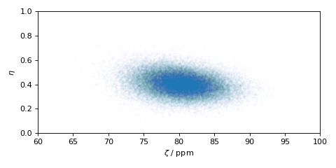
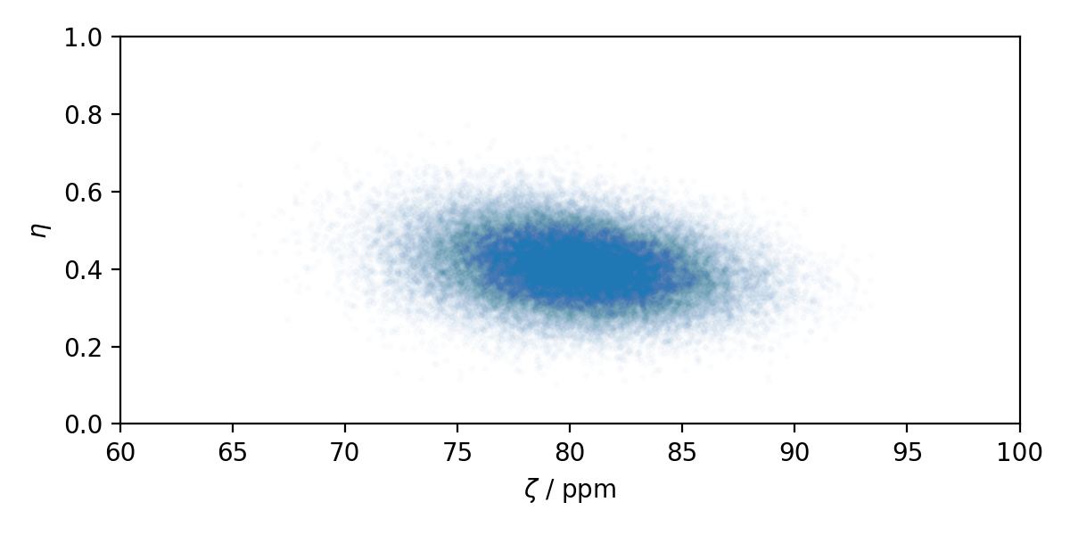
The scatter plot of these coordinates is shown below.
import matplotlib.pyplot as plt

plt.scatter(zeta_dist, eta_dist, s=4, alpha=0.01)
plt.xlabel("$\\zeta$ / ppm")
plt.ylabel("$\\eta$")
plt.xlim(60, 100)
plt.ylim(0, 1)
plt.tight_layout()
plt.show()

Figure 18 Extended Czjzek Distribution of shielding tensors.
Extended Czjzek distribution of symmetric quadrupolar tensors
The extended Czjzek distribution of symmetric quadrupolar tensors follows a similar
setup as the extended Czjzek distribution of symmetric shielding tensors, shown above.
In the following example, we generate the probability distribution
function using the pdf() method.
import numpy as np

Cq_range = np.linspace(2, 6, num=100)  # pre-defined Cq range in MHz.
eta_range = np.linspace(0, 1, num=20)  # pre-defined eta range.

quad_tensor = {"Cq": 3.5, "eta": 0.23}  # Cq assumed in MHz
model_quad = ExtCzjzekDistribution(quad_tensor, eps=0.2)
Cq_grid, eta_grid, amp = model_quad.pdf(pos=[Cq_range, eta_range], size=400000)
As with the case of the Czjzek distribution, to generate a probability distribution of the
extended Czjzek distribution, we need to define a grid system over which the distribution
probabilities will be evaluated. We do so by defining the range of coordinates along the
two dimensions. In the above example, Cq_range and eta_range are the
range of \(\text{Cq}\) and \(\eta_q\) coordinates, which is then given as the
argument to the pdf() method. The pdf
method also accepts the keyword argument size which defines the number of random samples
to approximate the probability distribution. A larger number will create better
approximations, although this increased quality comes at the expense of computation time.
The output Cq_grid, eta_grid, and amp hold the two coordinates and
amplitude, respectively.
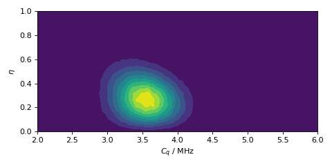
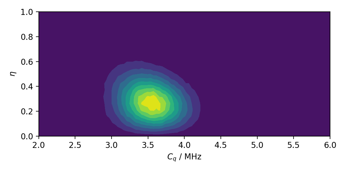
The plot of the extended Czjzek probability distribution is shown below.
import matplotlib.pyplot as plt

plt.contourf(Cq_grid, eta_grid, amp, levels=10)
plt.xlabel("$C_q$ / MHz")
plt.ylabel("$\\eta$")
plt.tight_layout()
plt.show()

Figure 20 Extended Czjzek Distribution of EFG tensors.
Extended Czjzek distribution in polar coordinates
As with the Czjzek distribution, we can sample an Extended Czjzek distribution on a polar
(x, y) grid. Below, we construct two equivalent
ExtCzjzekDistribution instances, except one is defined in polar
coordinates.
quad_tensor = {"Cq": 4.2, "eta": 0.15}  # Cq assumed in MHz
ext_cz_model = ExtCzjzekDistribution(quad_tensor, eps=0.4)
ext_cz_model_polar = ExtCzjzekDistribution(quad_tensor, eps=0.4, polar=True)

# Distribution in cartesian (zeta, eta) coordinates
Cq_range = np.linspace(2, 8, num=50)
eta_range = np.linspace(0, 1, num=20)
Cq_grid, eta_grid, amp = ext_cz_model.pdf(pos=[Cq_range, eta_range], size=2000000)

# Distribution in polar coordinates
x_range = np.linspace(0, 6, num=36)
y_range = np.linspace(0, 6, num=36)
x_grid, y_grid, amp_polar = ext_cz_model_polar.pdf(pos=[x_range, y_range], size=2000000)

# Plot the distributions
fig, ax = plt.subplots(1, 2, figsize=(9, 4), gridspec_kw={"width_ratios": (5, 4)})
ax[0].contourf(Cq_grid, eta_grid, amp, levels=10)
ax[0].set_xlabel("$C_q$ / MHz")
ax[0].set_ylabel("$\\eta$")
ax[0].set_title("Cartesian coordinates")
ax[1].contourf(x_grid, y_grid, amp_polar, levels=10)
ax[1].set_xlabel("x / MHz")
ax[1].set_ylabel("y / MHz")
ax[1].set_title("Polar coordinates")

plt.tight_layout()
plt.show()

Figure 22 Two equivalent Extended Czjzek distributions in Cartesian \(\left(\zeta, \eta\right)\) coordinates (left) and in polar \(\left(x, y\right)\) coordinates (right).
Note
The pdf method of the instance generates the probability distribution function
by first drawing random points from the distribution and then binning it
onto a pre-defined grid.
Mini-gallery using the extended Czjzek distributions
Extended Czjzek distribution (Shielding and Quadrupolar)
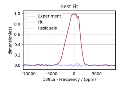
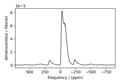
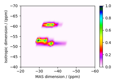
Extended Czjzek fitting of ¹³⁹La MAS NMR of La₀.₂Y₁.₈Si₂2O₇